Spotting Differences Among Observations

Marko Rak, Tim K

onig and Klaus-Dietz T

onnies

Department of Simulation and Graphics, Otto-von-Guericke University, Magdeburg, Germany

Keywords:

Density Difference, Kernel Density Estimation, Scale Space, Blob Detection, Afﬁne Shape Adaption.

Abstract:

Identifying differences among the sample distributions of different observations is an important issue in many

ﬁelds ranging from medicine over biology and chemistry to physics. We address this issue, providing a gen-

eral framework to detect difference spots of interest in feature space. Such spots occur not only at various

locations, they may also come in various shapes and multiple sizes, even at the same location. We deal with

these challenges in a scale-space detection framework based on the density function difference of the obser-

vations. Our framework is intended for semi-automatic processing, providing human-interpretable interest

spots for further investigation of some kind, e.g., for generating hypotheses about the observations. Such in-

terest spots carry valuable information, which we outline at a number of classiﬁcation scenarios from UCI

Machine Learning Repository; namely, classiﬁcation of benign/malign breast cancer, genuine/forged money

and normal/spondylolisthetic/disc-herniated vertebral columns. To this end, we establish a simple decision

rule on top of our framework, which bases on the detected spots. Results indicate state-of-the-art classiﬁcation

performance, which underpins the importance of the information that is carried by these interest spots.

1 INTRODUCTION

Sooner or later a large portion of pattern recognition

tasks come down to the question What makes X dif-

ferent from Y ? Some scenarios of that kind are:

Detection of forged money based on image-

derived features: What makes some sort of

forgery different from genuine money?

Comparison of medical data of healthy and

non-healthy subjects for disease detection:

What makes data of the healthy different from

that of the non-healthy?

Comparison of document data sets for text re-

trieval purposes: What makes this set of docu-

ments different from another set?

Apart from this, spotting differences in two or more

observations is of interest in ﬁelds of computational

biology, chemistry or physics. Looking at it from a

general perspective, such questions generalize to

What makes the samples of group X different

from the samples of group Y ?

This question usually arises when we deal with

grouped samples in some feature space. For humans,

answering such questions tends to become more chal-

lenging with increasing number of groups, samples

and feature space dimensions, up to the point where

we miss the forest for the trees. This complexity is

not an issue to automatic approaches, which, on the

other hand, tend to either overﬁt or underﬁt patterns

in the data. Therefore, semi-automatic approaches are

needed to generate a number of interest spots which

are to be looked at in more detail.

We address this issue by a scale-space difference

detection framework. Our approach relies on the den-

sity difference of group samples in feature space. This

enables us to identify spots where one group domi-

nates the other. We draw on kernel density estimators

to represent arbitrary density functions. Embedding

this into a scale-space representation, we are able to

detect spots of different sizes and shapes in feature

space in an efﬁcient manner. Our framework:

• applies to d-dimensional feature spaces¿

• is able to reﬂect arbitrary density functions

• selects optimal spot locations, sizes and shapes

• is robust to outliers and measurement errors

• produces human-interpretable results

Our presentation is structured as follows. We out-

line the key idea of our framework in Section 2. The

speciﬁc parts of our framework are detailed in Sec-

tion 3, while Section 4 comprises our results on sev-

eral data sets. In Section 5, we close with a summary

of our work, our most important results and an outline

of future work.

Rak M., König T. and Tönnies K..

Spotting Differences Among Observations.

DOI: 10.5220/0005165300050013

In Proceedings of the International Conference on Pattern Recognition Applications and Methods (ICPRAM-2015), pages 5-13

ISBN: 978-989-758-076-5

 2015 SCITEPRESS (Science and Technology Publications, Lda.)

2 FOUNDATIONS

Searching for differences between the sample distri-

bution of two groups of observations g and h, we,

quite naturally, seek for spots where the density func-

tion f

(x) of group g dominates the density function

(x) of group h, or vice versa. Hence, we try to ﬁnd

positive-/negative-valued spots of the density differ-

ence

g−h

(x) = f

(x) − f

(x) (1)

w.r.t. the underlying feature space R

with x ∈ R

Such spots may come in various shapes and sizes. A

difference detection framework should be able to deal

with these degrees of freedom. Additionally, it must

be robust to various sources of error, e.g., from mea-

surement, quantization and outliers.

We propose to superimpose a scale-space repre-

sentation to the density difference f

g−h

(x) to achieve

the above-mentioned properties. Scale-space frame-

works have been shown to robustly handle a wide

range of detection tasks for various types of struc-

tures, e.g., text strings (Yi and Tian, 2011), per-

sons and animals (Felzenszwalb et al., 2010) in

natural scenes, neuron membranes in electron mi-

croscopy imaging (Seyedhosseini et al., 2011) or mi-

croaneurysms in digital fundus images (Adal et al.,

2014). In each of these tasks the function of interest

is represented through a grid of values, allowing for

an explicit evaluation of the scale-space. However, an

explicit grid-based approach becomes intractable for

higher-dimensional feature spaces.

In what follows, we show how a scale-space rep-

resenation of f

g−h

(x) can be obtained from kernel

density estimates of f

(x) and f

(x) in an implicit

fashion, expressing the problem by scale-space kernel

density estimators. Note that by the usage of kernel

density estimates our work is limited to feature spaces

with dense ﬁlling. We close with a brief discussion on

how this can be used to compare observations among

more than two groups.

2.1 Scale Space Representation

First, we establish a family l

g−h

(x;t) of smoothed ver-

sions of the densitiy difference l

g−h

(x). Scale param-

eter t ≥0 deﬁnes the amount of smoothing that is ap-

plied to l

g−h

(x) via convolution with kernel k

(x) of

bandwidth t as stated in

g−h

(x;t) = k

(x) ∗ f

g−h

(x). (2)

For a given scale t, spots having a size of about

√

t will be highlighted, while smaller ones will be

smoothed out. This leads to an efﬁcient spot detection

scheme, which will be discussed in Section 3. Let

(x;t) = k

(x) ∗ f

(x) (3)

(x;t) = k

(x) ∗ f

(x) (4)

be the scale-space representations of the group den-

sities f

(x) and f

(x). Looking at Equation 2 more

closely, we can rewrite l

g−h

(x;t) equivalently in terms

of l

(x;t) and l

(x;t) via Equation 3 and 4. This reads

g−h

(x;t) = k

(x) ∗ f

g−h

(x) (5)

= k

(x) ∗

(x) − f

(x)

(6)

= k

(x) ∗ f

(x) −k

(x) ∗ f

(x) (7)

= l

(x;t) −l

(x;t). (8)

The simple yet powerful relation between the left

and the right-hand side of Equation 8 will allow us

to evaluate the scale-space representation l

g−h

(x) im-

plicitly, i.e., using only kernel functions. Of major im-

portance is the choice of the smoothing kernel k

(x).

According to scale-space axioms, k

(x) should suf-

ﬁce a number of properties, resulting in the uniform

Gaussian kernel of Equation 9 as the unique choice,

cf. (Babaud et al., 1986; Yuille and Poggio, 1986).

(x) =

(2πt)

exp



−



(9)

2.2 Kernel Density Estimation

In kernel density estimation, the group density f

(x)

is estimated from its n

samples by means of a ker-

nel function K

(x). Let x

∈ R

d×1

with i = 1, . . . , n

being the group samples. Then, the group density es-

timate is given by

(x) =

∑

i=1



x −x



. (10)

Parameter B

∈ R

d×d

is a symmetric positive deﬁnite

matrix, which controls the inﬂuences of samples to

the density estimate. Informally speaking, K

(x) ap-

plies a smoothing with bandwidth B

to the “spiky

sample relief” in feature space.

Plugging kernel density estimator

(x) into the

scale-space representation l

(x;t) deﬁnes the scale-

space kernel density estimator

(x;t) to be

(x;t) = k

(x) ∗

(x). (11)

Inserting Equation 10 into the above, we can trace

down the deﬁnition of the scale-space density estima-

ICPRAM2015-InternationalConferenceonPatternRecognitionApplicationsandMethods

tor

(x;t) to the sample level via transformation

(x;t) = k

(x) ∗

(x) (12)

= k

(x) ∗

∑

i=1



x −x



(13)

∑

i=1

∗K

)



x −x



. (14)

Though arbitrary kernels can be used, we choose

(x) to be a Gaussian kernel Φ

(x) due to its con-

venient algebraic properties. This (potentially non-

uniform) kernel is deﬁned as

(x) =

det(2πB)

exp



−

−1



. (15)

Using the above, the right-hand side of Equa-

tion 14 simpliﬁes further because of the Gaussian’s

cascade convolution property. Eventually, the scale-

space kernel density estimator

(x;t) is given by

Equation 16, where I ∈ R

d×d

is the identity.

(x;t) =

∑

i=1

tI+B



x −x



(16)

Using this estimator, the scale-space representa-

tion l

(x;t) of group density f

(x) and analogously

that of group h can be estimated for any (x;t) in an

implicit fashion. Consequently, this allows us to es-

timate the scale-space representation l

g−h

(x;t) of the

density difference f

g−h

(x) via Equation 7 by means

of kernel functions only.

2.3 Bandwidth Selection

When regarding bandwidth selection in such a scale-

space representation, we see that the impact of differ-

ent choices for bandwidth matrix B vanishes as scale t

increases. This can be seen when comparing matrices

tI + 0 and tI + B where 0 represents the zero matrix,

i.e., no bandwidth selection at all. We observe that

relative differences between them become neglectable

once ktIk  kBk. This is especially true for large

sample sizes, because the bandwidth will then tend

towards zero for any reasonable bandwidth selector

anyway. Hence, we may actually consider setting B

to 0 for certain problems, as we typically search for

differences that fall above some lower bound for t.

Literature bares extensive work on bandwidth ma-

trix selection, for example, based on plug-in es-

timators (Duong and Hazelton, 2003; Wand and

Jones, 1994) or biased, unbiased and smoothed cross-

validation estimators (Duong and Hazelton, 2005;

Sain et al., 1992). All of these integrate well with our

scale-space density difference framework. However,

in view of the argument above, we propose to compro-

mise between a full bandwidth optimization and hav-

ing no bandwidth at all. We deﬁne B

= b

I and use

an unbiased least-squares cross-validation to set up

the bandwidth estimate for group g. For Gaussian ker-

nels, this leads to the optimization of 17, cf. (Duong

and Hazelton, 2005), which we achieved by golden

section search over b

argmin

det(4πB

)

−1)

∑

i=1

∑

j=1

j6=i

(Φ

−2Φ

)(x

−x

) (17)

2.4 Multiple Groups

If differences among more than two groups shall be

detected, we can reduce the comparison to a number

of two-group problems. We can consider two typi-

cal use cases, namely one group vs. another and one

group vs. rest. Which of the two is more suitable de-

pends on the speciﬁc task at hand. Let us illustrate

this using two medical scenarios. Assume we have

a number of groups which represent patients having

different diseases that are hard to discriminate in dif-

ferential diagnosis. Then we may consider the second

use case, to generate clues on markers that make one

disease different from the others. In contrast, if these

groups represent stages of a disease, potentially in-

cluding a healthy control group, then we may consider

the ﬁrst use case, comparing only subsequent stages

to give clues on markers of the disease’s progress.

3 METHOD

To identify the positve-/negative-valued spots of a

density difference, we apply the concept of blob de-

tection, which is well-known in computer vision, to

the scale-space representation derived in Section 2.

In scale-space blob detection, some blobness criterion

is applied to the scale-space representation, seeking

for local optima of the function of interest w.r.t. space

and scale. This directly leads to an efﬁcient detection

scheme that identiﬁes a spot’s location and size. The

latter corresponds to the detection scale.

In a grid-representable problem we can evaluate

blobness densely over the scale-space grid and iden-

tify interesting spots directly using the grid neigh-

borhood. This is intractable here, which is why we

rely on a more reﬁned three-stage approach. First, we

trace the local spatial optima of the density difference

SpottingDifferencesAmongObservations

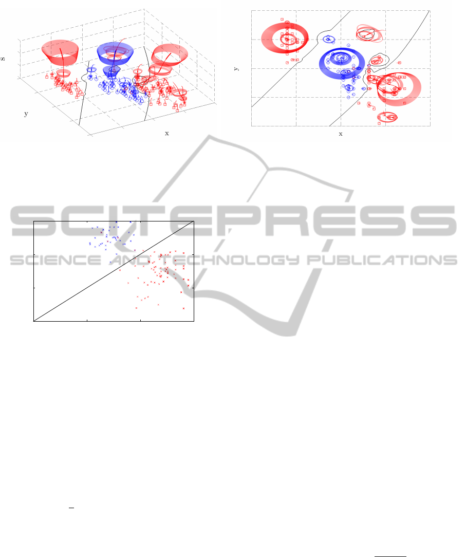
(a) “Isometric” View (b) Top View

Figure 1: Detection results for a two-group (red/blue) problem in two-dimensional feature space (xy-plane) with augmented

scale dimension s; Red squares and blue circles visualize the samples of each group; Red/blue paths outline the dendrogram of

scale-space density difference optima for the red/blue group dominating the other group; Interesting spots of each dendrogram

are printed thick; Red/blue ellipses characterize the shape for each of the interest spots.

through scales of the scale-space representation. Sec-

ond, we identify the interesting spots by evaluating

their blobness along the dendrogram of optima that

was obtained during the ﬁrst stage. Having selected

spots and therefore knowing their locations and sizes,

we ﬁnally calculate an elliptical shape estimate for

each spot in a third stage.

Spots obtained in this fashion characterize ellipti-

cal regions in feature space as outlined in Figure 1.

The representation of such regions, i.e., location, size

and shape, as well as its strength, i.e., its scale-space

density difference value, are easily interpretable by

humans, which allows to look at them in more detail

using some other method. This also renders a limita-

tion of our work, because non-elliptical regions may

only be approximated by elliptical ones. We now give

a detailed description of the three stages.

3.1 Scale Tracing

Assume we are given an equidistant scale sampling,

containing non-negative scales t

, . . . , t

in increasing

order and we search for spots where group g dom-

inates h. More precisely, we search for the non-

negatively valued maxima of l

g−h

(x;t

i−1

). The op-

posite case, i.e., group h dominates g, is equivalent.

Let us further assume that we know the spatial lo-

cal maxima of the density difference l

g−h

(x;t

i−1

) for

a certain scale t

i−1

and we want to estimate those of

the current scale t

. This can be done taking the previ-

ous local maxima as initial points and optimizing each

w.r.t. l

g−h

(x;t

). In the ﬁrst scale, we take the sam-

ples of group g themselves. As some maxima may

be converged to the same location, we merge them

together, feeding unique locations as initials into the

next scale t

i+1

only. We also drop any negatively-

valued locations as these are not of interest to our

task. They will not become of interest for any higher

scale either, because local extrema will not enhance as

scale increases, cf. (Lindeberg, 1998). Since deriva-

tives are simple to evaluate for Gaussian kernels, we

can use Newton’s method for spatial optimization.

We can assemble gradient

∂

∂x

g−h

(x;t) and Hessian

∂

∂x∂x

g−h

(x;t) sample-wise using

∂

∂x

(x) = −Φ

(x)B

−1

x and (18)

∂

∂x∂x

(x) = Φ

(x)



−1

−B

−1



. (19)

Iterating this process through all scales, we form

a discret dendrogram of the maxima over scales. A

dendrogram branching means that a maxima formed

from two (or more) maxima from the preceding scale.

3.2 Spot Detection

The maxima of interest are derived from a scale-

normalized blobness criterion c

(x;t). Two main cri-

teria, namely the determinant of the Hessian (Bret-

zner and Lindeberg, 1998) and the trace of the Hes-

sian (Lindeberg, 1998) have been discussed in litera-

ture. We focus on the former, which is given in Equa-

tion 20

, as it has been shown to provide better scale

selection properties under afﬁne transformation of the

feature space, cf. (Lindeberg, 1998).

(x;t) = t

γd

(−1)

det



∂

∂x∂x

g−h

(x;t)



| {z }

(20)

= t

γd

c(x;t) (21)

(−1)

handles even and odd dimensions consistently.

ICPRAM2015-InternationalConferenceonPatternRecognitionApplicationsandMethods

Because the maxima are already spatially optimal, we

can search for spots that maximize c

(x;t) w.r.t. the

dendrogram neighborhood only. Parameter γ ≥ 0 can

be used to introduce a size bias, shifting the detected

spot towards smaller or larger scales. The deﬁnition

of γ highly depends on the type of spot that we are

looking for, cf. (Lindeberg, 1996). This is impractical

when we seek for spots of, for example, small and

large skewness or extreme kurtosis at the same time.

Addressing the parameter issue, we search for

all spots that maximize c

(x;t) locally w.r.t. some

γ ∈ [0, ∞). Some dendrogram spot s with scale-space

coordinates (x

) is locally maximal if there exists

a γ-interval such that its blobness c

) is larger

than that of every spot in its dendrogram neighbor-

hood N (s). This leads to a number of inequalities,

which can be written as

γd

c(x

) >

∀n∈N (s)

γd

c(x

) or (22)

γd log

∀n∈N (s)

log

c(x

)

c(x

)

. (23)

The latter can be solved easily for the γ-interval, if

any. We can now identify our interest spots by look-

ing for the maxima along the dendrogram that locally

maximize the width of the γ-interval. More precisely,

let w

) be the width of the γ-interval for dendro-

gram spot s, then s is of interest if the dendrogram

Laplacian of w

(x;t) is negative at (x

), or equiva-

lently, if

) >



N (s)



∑

n∈N (s)

). (24)

Intuitively, a spot is of interest if its γ-interval width

is above neighborhood average. This is the only as-

sumption we can make without imposing limitations

on the results. Interest spots indentiﬁed in this way

will be dendrogram segments, each ranging over a

number of consecutive scales.

3.3 Shape Adaption

Shape estimation can be done in an iterative manner

for each interest spot. The iteration alternatingly up-

dates the current shape estimate based on a measure

of anisotropy around the spot and then corrects the

bandwidth of the scale-space smoothing kernel ac-

cording to this estimate, eventually reaching a ﬁxed

point. The second moment matrix of the function of

interest is typically used as an anisotropy measure,

e.g., in (Lindeberg and Garding, 1994) and (Mikola-

jczyk and Schmid, 2004). Since it requires spatial in-

tegration of the scale-space representation around the

interest spot, this measure is not feasible here.

We adapted the Hessian-based approach of (Lake-

mond et al., 2012) to d-dimensional problems.

The aim is to make the scale-space representation

isotropic around the interest spot, iteratively mov-

ing any anisotropy into the symmetric positive deﬁ-

nite shape matrix S ∈R

d×d

of the smoothing kernel’s

bandwidth tS. Thus, we lift the problem into a gen-

eralized scale-space representation l

g−h

(x;tS) of non-

uniform scale-space kernels, which requires us to re-

place the deﬁnition of φ

(x) by that of Φ

(x).

Starting with the isotropic S

= I, we decompose

the current Hessian via

∂

∂x∂x

g−h

(·;tS

) = VD

(25)

into its eigenvectors in columns of V and eigenvalues

on the diagonal of D

. We then normalize the latter to

unit determinant via

D =

det(D)D (26)

to get a relative measure of anisotropy for each of

the eigenvector directions. Finally, we move the

anisotropy into the shape estimate via

i+1



−





−



(27)

and start all over again. Iteration terminates when

isotropy is reached. More precisely: when the ratio

of minimal and maximal eigenvalue of the Hessian

approaches one, which usually happens within a few

iterations.

4 EXPERIMENTS

We next demonstrate that interest spots carry valuable

information about a data set. Due to the lack of data

sets that match our particular detection task a ground

truth comparison is impossible. Certainly, artiﬁcially

constructed problems are an exception. However, the

generalizability of results is at least questionable for

such problems. Therefore, we chose to benchmark

our approach indirectly via a number of classiﬁcation

tasks. The rational is that results that are comparable

to those of well-established classiﬁers should under-

pin the importance of the identiﬁed interest spots.

We next show how to use these interest spots for

classiﬁcation using a simple decision rule and detail

the data sets that were used. We then investigate pa-

rameters of our approach and discuss the results of the

classiﬁcation tasks in comparison to decision trees,

Fisher’s linear discriminant analysis, k-nearest neigh-

bors with optimized k and support vector machines

with linear and cubic kernels. All experiments were

performed via leave-one-out cross-validation.

SpottingDifferencesAmongObservations

(a) “Isometric” View (b) Top View

Figure 2: Feature space decision boundaries (black plane curves) obtained from group likelihood criterion for the two-

dimensional two-group problem of Figure 1; Red squares and blue circles visualize the samples of each group; Red/blue

paths outline the dendrogram of scale-space density difference optima for the red/blue group dominating the other group;

Interesting spots of each dendrogram are printed thick; Red/blue ellipses characterize the shape for each of the interest spots.

−6

−4

−2

−6

−4

−2

red

blue

Figure 3: Sample group likelihoods and decision boundary

(black diagonal line) for the two-group problem of Figure 1.

4.1 Decision Rule

To perform classiﬁcation we establish a simple deci-

sion rule based on interest spots that were detected us-

ing the one group vs. rest use case. Therefore, we de-

ﬁne a group likelihood criterion as follows. For each

group g, having the set of interest spots I

, we deﬁne

(x) = max

s∈I

g−h

)

·exp



−

(x −x

)

−1

(x −x

)



. (28)

This is a quite natural trade-off, where the ﬁrst factor

favors spots s with high density difference, while the

latter factor favors spots with small Mahalanobis dis-

tance to the location x that is investigated. We may

also think of p

(x) as an exponential approximation

of the scale-space density difference using interesting

spots only. Given this, our decision rule simply takes

the group that maximizes the group likelihood for the

location of interest x. Figure 2 and Figure 3 illustrate

the decision boundary obtained from this rule.

4.2 Data Sets

We carried out our experiments on three classiﬁ-

cation data sets taken from UCI Machine Learn-

ing Repository. A brief summary of them is given

in Table 1. In the ﬁrst task, we distinguish be-

tween benign and malign breast cancer based on

manually graded cytological charateristics, cf. (Wol-

berg and Mangasarian, 1990). In the second task,

we distinguish between genuine and forged money

based on wavelet-transform-derived features from

photographs of banknote-like specimen, cf. (Glock

et al., 2009). In the third task, we differentiate among

normal, spondylolisthetic and disc-herniated vertebral

columns based on biomechanical attributes derived

from shape and orientation of the pelvis and the lum-

bar vertebral column, cf. (Berthonnaud et al., 2005).

4.3 Parameter Investigation

Before detailing classiﬁcation results, we investigate

two aspects of our approach. Firstly, we inspect

the importance of bandwidth selection, benchmarking

no kernel density bandwidth against the least-squares

cross-validation technique that we use. Secondly, we

determine the inﬂuence of the scale sampling rate.

For the latter we space n + 1 scales for various n

equidistantly from zero to

= F

−1

(1 −ε|d) max



det(Σ

)



, (29)

where F

−1

(·|d) is the cumulative inverse-χ

distribu-

tion with d degrees of freedom and Σ

is the covari-

ance matrix of group g. Intuitively, t

captures the

extent of the group with largest variance up to a small

ε, i.e., here 1.5 ·10

−8

ICPRAM2015-InternationalConferenceonPatternRecognitionApplicationsandMethods

Table 1: Data sets from UCI Machine Learning Repository.

Breast Cancer (BC) Banknote Authentication Vertebral Column

Groups benign / malign genuine / forged normal / spondylolisthetic / herniated discs

Samples 444 / 239 762 / 610 100 / 150 / 60

Dimensions 10 4 6

Table 2: Classiﬁcation accuracy of our decision rule in b%c for data sets of Table 1 with/without bandwidth selection.

Scale sampling rate n

100 125 150 175 200 225 250 270 300

Breast Cancer 65 / 65 97 / 97 97 / 97 95 / 95 97 / 97 95 / 95 97 / 97 96 / 96 97 / 97

Banknote Authen. 96 / 94 96 / 96 96 / 96 98 / 98 98 / 98 98 / 98 98 / 98 98 / 98 99 / 99

Vertebral Column 87 / 82 88 / 83 88 / 84 88 / 83 88 / 85 88 / 85 88 / 86 88 / 86 88 / 87

To investigate the two aspects, we compare classi-

ﬁcation accuracies with and without bandwidth selec-

tion as well as sampling rates ranging from n = 100

to n = 300 in steps of 25. From the results, which are

given in Table 2, we observe that bandwidth selection

is almost neglectable for the Breast Cancer (BC) and

the Banknote Authentication (BA) data set. However,

the impact is substantial throughout all scale sampling

rates for the Vertebral Column (VC) data set. This

may be due to the comparably small number of sam-

ples per group for this data set. Regarding the sec-

ond aspect, we observe that for the BA and VC data

set the classiﬁcation accuracy slightly increases when

the scale sampling rate rises. Regarding the BC data

set, accuracy remains relatively stable, except for the

lower rates. From the results we conclude that band-

width selection is a necessary part for interest spot

detection. We further recommend n ≥ 200, because

accuracy starts to saturate at this point for all data sets.

For the remaining experiments we used bandwidth se-

lection and a sampling rate of n = 200.

4.4 Classiﬁcation Results

A comparison of classiﬁcation accuracies of our de-

cision rule against the aforementioned classiﬁers is

given in Table 3. For the BC data set we observe that

except for the support vector machine (SVM) with cu-

bic kernel all approaches were highly accurate, scor-

ing between 94% and 97% with our decision rule be-

ing topmost. Even more similar to each other are re-

sults for the BA data set, where all approaches score

between 97% and 99%, with ours lying in the middle

of this range. Results are most diverse for the VC data

sets. Here, the SVM with cubic kernel again performs

signiﬁcantly worse than the rest, which all score be-

tween 80% and 85%, while our decision rule peaks

at 88%. Other research showed similar scores on the

given data sets. For example the artiﬁcial neural net-

works based on pareto-differential evolution in (Ab-

Table 3: Classiﬁcation accuracies of different classiﬁers in

b%c for data sets of Table 1.

BC BA VC

decision tree 94 98 82

k-nearest neighbors 97 99 80

Fisher’s discriminant 96 97 80

linear kernel SVM 96 99 85

cubic kernel SVM 90 98 74

our decision rule 97 98 88

bass, 2002) obtained 98% accuracy for the BC data

set, while (Rocha Neto et al., 2011) achieved 83% to

85% accuracy on the VC data set with SVMs with dif-

ferent kernels. These results suggest that our interest

points carry information about a data set that are sim-

ilarly important than the information carried by the

well-established classiﬁers.

Confusion tables for our decision rule are given

in Table 4 for all data sets. As can be seen, our ap-

proach gave balanced inter-group results for the BC

and the BA data set. We obtained only small inac-

curacies for the recall of the benign (96%) and gen-

uine (97%) groups as well as for the precision of the

malign (94%) and forged (96%) groups. Results for

the VC data set were more diverse. Here, a num-

ber of samples with disc herniation were mistaken

for being normal, lowering the recall of the herniated

group (86%) noticeably. However, more severe inter-

group imbalances were caused by the normal sam-

ples, which were relatively often mistaken for being

spondylolisthetic or herniated discs. Thus, recall for

the normal group (76%) and precision for the herni-

ated group (74%) decreased signiﬁcantly. The latter is

to some degree caused by a handful of strong outliers

from the normal group that fall into either of the other

groups, which can already be seen from the group

likelihood plot in Figure 4. This ﬁnding was made by

others as well, cf. (Rocha Neto and Barreto, 2009).

The other classiﬁers performed similarly balanced

on the BA and BC data set. Major differences occured

SpottingDifferencesAmongObservations

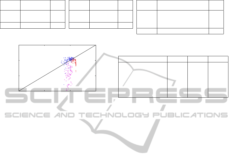
Table 4: Confusion table for predicted/actual groups of our decision rule for data sets of Table 1.

(a) Breast Cancer

ben. mal.

ben. 429 4 99

mal. 15 235 94

96 98 b%c

(b) Banknote Authentication

gen. for.

gen. 742 0 100

for. 20 610 96

97 100 b%c

norm. spon. hern.

norm. 76 1 6 91

spon. 10 145 2 92

hern. 14 4 52 74

76 96 86 b%c

−30

−20

−10

−30

−20

−10

max

spond.

, p

hern.

normal

Figure 4: Sample group likelihoods and decision boundary

(black diagonal line) for the Vertebral Column data set of

Table 1; Normal, spondylolisthetic and herniated discs in

blue, magenta and red, respectively.

on the VC data set only. A precision/recall compar-

ison of all classiﬁers on the VC data set is given in

Table 5. We observe that the precision of the normal

and the herniated group are signiﬁcantly lower (gap >

12%) than that of the spondylolisthetic group for all

classiﬁers except for our decision rule, for which at

least the normal group is predicted with a similar pre-

cision. Regarding the recall we note an even more

unbalanced behavior. Here, a strict ordering from

spondylolisthetic over normal to herniated disks oc-

curs. The differences of the recall of spondylolisthetic

and normal are signiﬁcant (gap > 16 %) and those

between normal and herniated are even larger (gap >

18 %) among all classiﬁers that we compared against.

The recalls for our decision rule are distributed differ-

ently, ordering the herniated before the normal group.

Also the magnitude of differences is less signiﬁcant

(gaps ≈ 10%) for our decision rule. Results of this

comparison indicate that the information that is car-

ried by our interest points tends to be more balanced

among groups than the information carried by the

well-established classiﬁers that we compared against.

5 CONCLUSION

We proposed a detection framework that is able to

identify differences among the sample distributions

of different observations. Potential applications are

Table 5: Classiﬁcation precision/recall of different classi-

ﬁers in b%c for the Vertebral Column data set of Table 1.

norm. spon. hern.

decision tree 69 / 83 97 / 95 68 / 50

k-nearest neighbors 70 / 74 96 / 96 58 / 55

Fisher’s discriminant 70 / 80 87 / 92 74 / 48

linear kernel SVM 76 / 85 97 / 96 72 / 61

cubic kernel SVM 59 / 82 90 / 91 52 / 18

our decision rule 91 / 76 92 / 96 74 / 86

manifold, touching ﬁelds such as medicine, biology,

chemistry and physics. Our approach bases on the

density function difference of the observations in fea-

ture space, seeking to identify spots where one obser-

vation dominates the other. Superimposing a scale-

space framework to the density difference, we are able

to detect interest spots of various locations, size and

shapes in an efﬁcient manner.

Our framework is intended for semi-automatic

processing, providing human-interpretable interest

spots for potential further investigation of some kind.

We outlined that these interest spots carry valuable

information about a data set at a number of classiﬁ-

cation tasks from the UCI Machine Learning Repos-

itory. To this end, we established a simple decision

rule on top of our framework. Results indicate state-

of-the-art performance of our approach, which under-

pins the importance of the information that is carried

by these interest spots.

In the future, we plan to extend our work to sup-

port repetitive features such as angles, which cur-

rently is a limitation of our approach. Modifying our

notion of distance, we would then be able to cope with

problems deﬁned on, e.g., a sphere or torus. Future

work may also include the migration of other types of

scale-space detectors to density difference problems.

This includes the notion of ridges, valleys and zero-

crossings, leading to richer sources of information.

ACKNOWLEDGEMENTS

This research was partially funded by the project “Vi-

sual Analytics in Public Health” (TO 166/13-2) of the

ICPRAM2015-InternationalConferenceonPatternRecognitionApplicationsandMethods

German Research Foundation.

REFERENCES

Abbass, H. A. (2002). An evolutionary artiﬁcial neural net-

works approach for breast cancer diagnosis. Artiﬁcial

Intelligence in Medicine, 25:265–281.

Adal, K. M., Sidibe, D., Ali, S., Chaum, E., Karnowski,

T. P., and Meriaudeau, F. (2014). Automated detection

of microaneurysms using scale-adapted blob analysis

and semi-supervised learning. Computer Methods and

Programs in Biomedicine, 114:1–10.

Babaud, J., Witkin, A. P., Baudin, M., and Duda, R. O.

(1986). Uniqueness of the Gaussian kernel for scale-

space ﬁltering. IEEE Transactions on Pattern Analysis

and Machine Intelligence, 8:26–33.

Berthonnaud, E., Dimnet, J., Roussouly, P., and Labelle,

H. (2005). Analysis of the sagittal balance of the

spine and pelvis using shape and orientation param-

eters. Journal of Spinal Disorders and Techniques,

18:40–47.

Bretzner, L. and Lindeberg, T. (1998). Feature tracking with

automatic selection of spatial scales. Computer Vision

and Image Understanding, 71:385–392.

Duong, T. and Hazelton, M. L. (2003). Plug-in bandwidth

matrices for bivariate kernel density estimation. Jour-

nal of Nonparametric Statistics, 15:17–30.

Duong, T. and Hazelton, M. L. (2005). Cross-validation

bandwidth matrices for multivariate kernel density es-

timation. Scandinavian Journal of Statistics, 32:485–

506.

Felzenszwalb, P. F., Girshick, R. B., McAllester, D., and

Ramanan, D. (2010). Object detection with discrim-

inatively trained part-based models. IEEE Transac-

tions on Pattern Analysis and Machine Intelligence,

32:1627–1645.

Glock, S., Gillich, E., Schaede, J., and Lohweg, V. (2009).

Feature extraction algorithm for banknote textures

based on incomplete shift invariant wavelet packet

transform. In Proceedings of the Annual Pattern

Recognition Symposium, volume 5748, pages 422–

431.

Lakemond, R., Sridharan, S., and Fookes, C. (2012).

Hessian-based afﬁne adaptation of salient local image

features. Journal of Mathematical Imaging and Vi-

sion, 44:150–167.

Lindeberg, T. (1996). Edge detection and ridge detection

with automatic scale selection. In Proceedings of the

IEEE Computer Society Conference on Computer Vi-

sion and Pattern Recognition, pages 465–470.

Lindeberg, T. (1998). Feature detection with automatic

scale selection. International Journal of Computer Vi-

sion, 30:79–116.

Lindeberg, T. and Garding, J. (1994). Shape-adapted

smoothing in estimation of 3-d depth cues from afﬁne

distortions of local 2-d brightness structure. In Pro-

ceedings of the European Conference on Computer

Vision, pages 389–400.

Mikolajczyk, K. and Schmid, C. (2004). Scale & afﬁne in-

variant interest point detectors. International Journal

of Computer Vision, 60:63–86.

Rocha Neto, A. R. and Barreto, G. A. (2009). On the appli-

cation of ensembles of classiﬁers to the diagnosis of

pathologies of the vertebral column: A comparative

analysis. IEEE Latin America Transactions, 7:487–

496.

Rocha Neto, A. R., Sousa, R., Barreto, G. A., and Cardoso,

J. S. (2011). Diagnostic of pathology on the verte-

bral column with embedded reject option. In Pattern

Recognition and Image Analysis, volume 6669, pages

588–595. Springer Berlin Heidelberg.

Sain, S. R., Baggerly, K. A., and Scott, D. W. (1992). Cross-

validation of multivariate densities. Journal of the

American Statistical Association, 89:807–817.

Seyedhosseini, M., Kumar, R., Jurrus, E., Giuly, R., Ellis-

man, M., Pﬁster, H., and Tasdizen, T. (2011). De-

tection of neuron membranes in electron microscopy

images using multi-scale context and Radon-like fea-

tures. In Proceedings of the International Conference

on Medical Image Computing and Computer-assisted

Intervention, pages 670–677.

Wand, M. P. and Jones, M. C. (1994). Multivariate plug-in

bandwidth selection. Computational Statistics, 9:97–

116.

Wolberg, W. and Mangasarian, O. (1990). Multisurface

method of pattern separation for medical diagnosis ap-

plied to breast cytology. In Proceedings of the Na-

tional Academy of Sciences, pages 9193–9196.

Yi, C. and Tian, Y. (2011). Text string detection from natu-

ral scenes by structure-based partition and grouping.

IEEE Transactions on Image Processing, 20:2594–

2605.

Yuille, A. L. and Poggio, T. A. (1986). Scaling theorems for

zero crossings. IEEE Transactions on Pattern Analy-

sis and Machine Intelligence, 8:15–25.

SpottingDifferencesAmongObservations

REFERENCES

Abbass, H. A. (2002). An evolutionary artificial neural net-