Improved Confidence Measures for Variational Optical Flow
Maren Brumm, Jan Marek Marcinczak and Rolf-Rainer Grigat
TU Hamburg-Harburg, Harburger Schlossstraße 20, 21079 Hamburg, Germany
Keywords:
Variational Optical Flow, Confidence Measure, Performance Evaluation, Structure-Texture Decomposition.
Abstract:
In the last decades variational optical flow algorithms have been intensively studied by the computer vision
community. However, relatively few effort has been made to obtain robust confidence measures for the es-
timated flow field. As many applications do not require the whole flow field, it would be helpful to identify
the parts of the field where the flow is most accurate. We propse a confidence measure based on the energy
functional that is minimized during the optical flow calculation and analyze the performance of different data
terms. For evaluation, 7 datasets of the Middlebury benchmark are used. The results show that the accuracy of
the flow field can be improved by 53.3 % if points are selected according to the proposed confidence measure.
The suggested method leads to an improvement of 35.2 % compared to classical confidence measures.
1 INTRODUCTION
Since Horn and Schunck (Horn and Schunck, 1981)
variational optical flow has been an active field of re-
search. An optical flow field gives for every pixel in
the first input image a motion vector that estimates
the movement to its new position in the second im-
age. There are many different applications for which
the optical flow field can be used, such as motion seg-
mentation or 3D reconstruction. However, the optical
flow estimation is difficult in areas with changing il-
lumination or complex movements. Commonly, there
are areas, where the flow field is less accurate than in
others. Many applications require the flow field only
for a subset of pixels. Therefore, a confidence mea-
sure is needed to identify the parts of the field where
the flow is most reliable. Another issue is continu-
ous tracking, where points are tracked over several
frames. Here, a confidence measure can be used to
detect vanishing points or poorly estimated points that
would lead to large errors if tracked on.
Barron et al. (Barron et al., 1994) proposed to use
the magnitude of the image gradient as confidence
measure. The intention is to reward high structure
image parts as the data term has very little informa-
tive value in image parts of low structure. However,
they demonstrated that this approach is not reliable
for variational methods. Bruhn and Weickert argue in
(Bruhn and Weickert, 2006) that large gradients com-
monly result from noise and from pixels that are oc-
cluded in the second frame, while areas with small
gradients might be filled in accurately by regulariza-
tion.
The approach described in (Bruhn and Weickert,
2006; Bruhn et al., 2005) uses the energy functional
that is minimized during the flow calculation as con-
fidence measure. The smaller the contribution of a
pixel to the final energy the more reliable it is rated.
In this paper we use a similar approach, but do
not limit ourself to using the same data term for the
confidence measure as for the optical flow estimation.
Instead we analyze the performance of linear and non-
linear data terms as well as different constancy as-
sumptions based on a structure-texture decomposi-
tion. We especially address the problem of changing
illumination by adding a data term that penalizes ar-
eas with high illumination changes.
For evaluation seven datasets with ground truth of
the Middlebury benchmark (Baker et al., 2011) are
used.
Future work will show whether additional im-
provements can be made by optimizing the weight-
ing between data term and regularization term and by
considering different norms on both terms.
2 OPTICAL FLOW ESTIMATION
Let I : Ω → R with Ω ⊂ R
2
be a greyscale image and
let (x, y) denote the image coordinates. For an im-
age pair I
1
(x, y) and I
2
(x, y) the optical flow u(x, y) =
(u, v) describes how the points move between I
1
(x, y)
and I
2
(x, y).
389
Brumm M., Marcinczak J. and Grigat R..
Improved Confidence Measures for Variational Optical Flow.
DOI: 10.5220/0005167203890394
In Proceedings of the 10th International Conference on Computer Vision Theory and Applications (VISAPP-2015), pages 389-394
ISBN: 978-989-758-091-8
Copyright
c
 2015 SCITEPRESS (Science and Technology Publications, Lda.)

The key assumption for the optical flow estimation is
that the grey value of a point in space is constant in
all frames. Classically, this constancy assumption is
given by (Horn and Schunck, 1981):
∂I(x, y, t)
∂t
= 0 . (1)
Following the description in (Wedel and Cremers,
2011, p. 9) it can be expressed as follows:
I
1
(x, y) = I
2
(x + u, y + v). (2)
Using the first taylor approximation of I
2
(x + u, y +v)
leads to
I
1
(x, y) = I
2
(x, y) + ∇I
2
(x, y)
T

u
v

, (3)
0 = I
2
(x, y) − I
1
(x, y)
| {z }
I
t
+∇I
2
(x, y)
T

u
v

. (4)
Denoting the partial derivatives with I
t
, I
x
and I
y
the
linearized optical flow constraint reads
0 = I
t
+ I
x
u + I
y
v. (5)
The optical flow constraint usually refers to the
constancy of the grey values in the input frames.
However, grey values are not illumination invariant.
Hence, we consider the use of other pixel properties,
see Section 4.
The given constraint leads to an under-determined
equation system and cannot be used solely to esti-
mate the optical flow field. Horn and Schunck (Horn
and Schunck, 1981) proposed to use the additional
assumption that the resulting flow field should be
smooth. This leads to the following minimization
problem:
min
u,v

Z
Ω
|∇u| + |∇v| + λ|I
t
+ I
x
u + I
y
v|dΩ

. (6)
The data term enforces the optical flow constraint,
while the regularization term favours smooth flow
fields by penalizing deviations in the flow flied. The
parameter λ weights between both terms. Commonly,
it is advisable to use the L
1
norm instead of the L
2
norm because it is discontinuity preserving and robust
to outliers (Zach et al., 2007).
3 CONFIDENCE MEASURE
The proposed confidence measure is based on the en-
ergy functional (6) that is minimized to obtain the op-
tical flow field. As described in (Bruhn and Weick-
ert, 2006) the underlying idea is that the flow field
is most accurate in those areas where the functional
has the lowest cost. However, there are different re-
quirements for the calculation of a flow field and the
rating of its accuracy. Therefore, we analyze different
energy formulations to include additional information
which supports classification.
Two different strategies are tested. The first is to
use exactly the same energy functional as confidence
measure that is used to estimate the optical flow:
e
lin
= |∇u| + |∇v| + λ
N
∑
i=1
|I
d
t
+ I
d
x
u + I
d
y
v|, (7)
where N denotes the number of constancy assump-
tions used in the data term and I
d
(x, y) denotes the
pixel property that is assumed to be constant. This
implies that the data term is linearized. As the esti-
mated flow is available, there is no need to linearize
the data term and the nonlinear data term |I
1
(x, y) −
I
2
(x + u, y + v)| can be calculated directly. Therefore,
the following confidence measure provides a higher
accuracy as it uses the optical flow constraint directly
instead of approximating it:
e
nonlin
= |∇u| + |∇v|+ λ
N
∑
i=1
|I
d
1
(x, y)−I
d
2
(x +u, y + v)|
(8)
Instead of limiting us to using the same constancy as-
sumption in the optical flow constraint for the con-
fidence measure as for the flow calculation, we also
consider other constancy assumptions for the confi-
dence measure, as described in the next section.
4 STRUCTURE-TEXTURE
DECOMPOSITION
Wedel and Cremer propose in (Wedel and Cremers,
2011, p. 36f) to perform a structure-texture decompo-
sition (Meyer, 2001) on the input images for the cal-
culation of the optical flow field. As shadows show up
mainly in the structural part, it increases the robust-
ness to illumination changes to assume the constancy
of the textural part only.
However, for the confidence measure both chan-
nels carry valuable information. The texture chan-
nel provides information on how well a pixel values
matches while the structure channel can be used to
filter out areas with significant illumination changes
where the optical flow is expected to be less reli-
able. Hence we consider using both the texture and
the structure channel for the confidence measure. By
decomposing the image and comparing both channels
separately additional information can be gained com-
pared to simply comparing the grey values without
VISAPP2015-InternationalConferenceonComputerVisionTheoryandApplications
390

decomposition.
The structural part I
S
(x) of the grey value image
I(x) is obtained by solving
min
I
S
Z
Ω
|∇I
s
(x)| +
1
2θ
(I
s
(x) − I(x))
2
dx . (9)
The solution to this problem can be found in (Wedel
and Cremers, 2011, p. 27f).
The textural part I
T
(x) can then be calculated by
I
T
(x) = I(x)− αI
S
(x). (10)
Parameters are set according to (Wedel and Cremers,
2011, p. 36f) to α = 0.95 and θ = 0.125 and 100
iterations are used to calculate I
S
.
5 EVALUATION
To evaluate the performance of the proposed con-
fidence measures, seven datasets of the Middlebury
benchmark (Baker et al., 2011) for which a ground
truth is available are used.
To measure the accuracy of an estimated optical
flow field, the end point error (Otte and Nagel, 1994)
is used. It is defined as
ε
∆
= ku − u
0
k, (11)
where u is the correct displacement vector and u
0
the
calculated displacement vector.
For evaluation the flow field of each dataset is
gradually filtered according to the confidence mea-
sure. The average end point error for the remaining
flow vectors is calculated in every step. For the cal-
culation of the optical flow field, the texture channel
is used in the data term unless stated otherwise. For
the energy functional a variety of different data terms
is considered. The weighting between regularization
term and data term for the confidence measure is set
to λ = 0.5 .
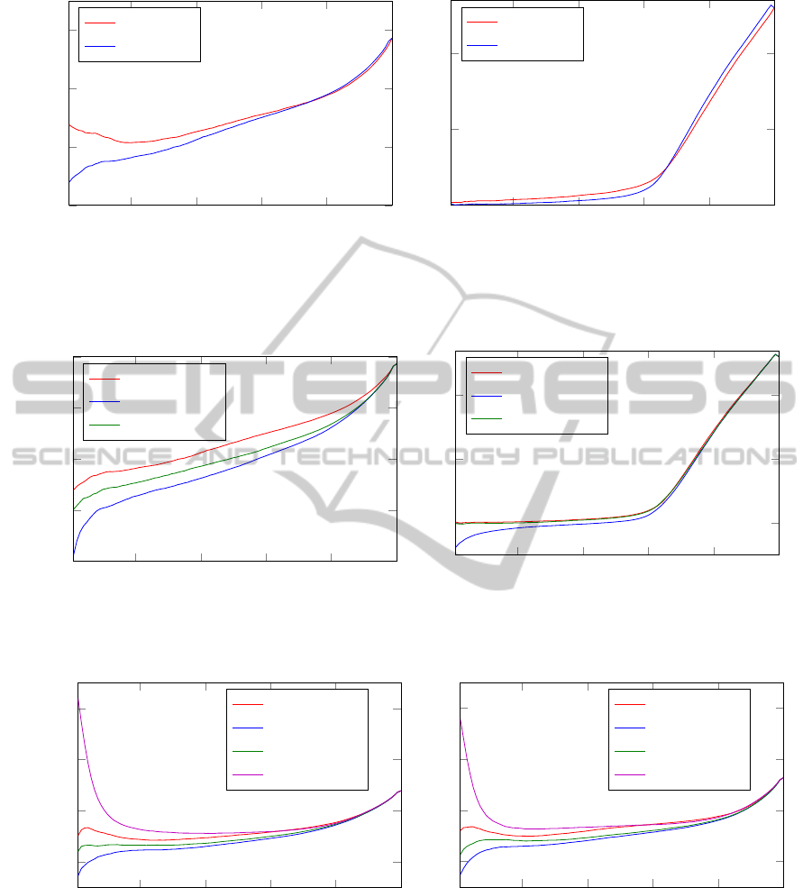
A comparison of the efficiency of the confidence
measures with a linear and a nonlinear data term for
two datasets of the Middlebury benchmark can be
seen in Figure 1. For both flow calculation and the
confidence measure the texture channel is used in
the data term. It can be seen that both confidence
measures are suitable to select points with low end
point error. For the dataset ’Grove2’ the linear and
nonlinear confidence measure give similar results for
selection rates of 75 % and more, although e
lin
can
reduce the error slightly more. For selection rates
below 75 % e
nonlin
is significantly more effective. It
decreases the error monotonically, while for e
lin
the
error rises again for selection rates below 18 %. For
the other dataset both confidence measures show a
similar performance. Both monotonically decrease
the error. For selection rates below 65 % e
nonlin
gives better results, for higher selection rates e
lin
gives better results. Overall e
nonlin
is more effective,
although e
lin
seems to be more suitable for high
selection rates. Taking all selection rates of both
datasets into account using the nonlinear data term
instead of the linear one improves the results on
average by 2.2 %. For a selection rate of 1 % the
average improvement is 7.6 %. Therefore, e
nonlin
is
used in the following evaluations.
Figure 2 displays the results of the confidence
measure e
nonlin
on the same datasets for three dif-
ferent data terms in the confidence measure. The
different data terms use a constancy assumption on
the grey value channel, the texture channel and both
the structure and texture channel. It can be seen
that the best results are obtained when not only the
texture channel of the images is used but the texture
and structure channel are used together. The structure
channel, which contains most of the shadow and
shading, may not be suitable to find a pixel matching
itself. Nevertheless, it gives valuable information on
how well the pixels are matched because in the areas
with significant illumination changes the optical flow
is expected to be less reliable. The structure-texture
data term also outperforms the grey value data term.
So apparently decomposing the image and compar-
ing the channels separately leads to a significant
improvement, especially for low selection rates.
For the dataset ’Grove2’ the end point error can be
reduced monotonically from 0.89 px to 0.51 px when
using only 1 % of the correspondences. This is an
improvement of 43 %. For the dataset ’Hydrangea’
the error can even be reduced by 83 %.
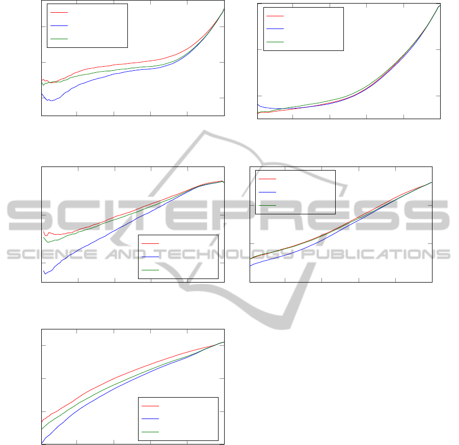
The results for five other datasets of the Middle-
bury benchmark can be seen in Figure 4. The
structure-texture data term gives the best results
for all datasets, except for ’RubberWhale’ where
using the texture channel only is most effective for
selection rates below 30 %. For higher selection rates
the structure-texture data term again gives the best
results. The end point error is reduced on average
over all datasets evaluated by 53.3 % if 1 % of the
flow field is selected. The average improvement over
all datasets tested for the structure-texture data term
compared to the grey value data term is 11.5 % for
a selection rate of 1 % and 3.8 % over all selection
rates.
Overall using the nonlinear structure-texture data
term improves the performance of the confidence
measure by 35.2 % for a selection rate of 1 % com-
pared to using exactly the same data term as for the
flow calculation.
ImprovedConfidenceMeasuresforVariationalOpticalFlow
391

20 40
60
80 100
0.6
0.7
0.8
0.9
points taken [%]
end point error [px]
e
lin
(I
T
)
e
nonlin
(I
T
)
(a) dataset ’Grove2’
20 40
60
80 100
0.1
0.2
0.3
points taken [%]
e
lin
(I
T
)
e
nonlin
(I
T
)
(b) dataset ’Hydrangea’
Figure 1: Comparison of the confidence measures with a linear and nonlinear data term for two sequences of the Middlebury
benchmark. For selection rates of 65% and lower the nonlinear data term gives better results.
20 40
60
80 100
0.5
0.6
0.7
0.8
0.9
points taken [%]
end point error [px]
e
nonlin
(I
T
)
e
nonlin
(I
T
, I
S
)
e
nonlin
(I
grey
)
(a) dataset ’Grove2
20 40
60
80 100
0.1
0.2
0.3
points taken [%]
e
nonlin
(I
T
)
e
nonlin
(I
T
, I
S
)
e
nonlin
(I
grey
)
(b) dataset ’Hydrangea’
Figure 2: Comparison of different constancy assumptions in the data term. e(I
T
, I
S
) shows the best results.
20 40
60
80 100
0.6
0.8
1
1.2
points taken [%]
end point error [px]
e
nonlin
(I
T
)
e
nonlin
(I
T
, I
S
)
e
nonlin
(I
grey
)
e
nonlin
(I
grad
)
(a) flow calculated with I
grey
20 40
60
80 100
0.6
0.8
1
1.2
points taken [%]
e
nonlin
(I
T
)
e
nonlin
(I
T
, I
S
)
e
nonlin
(I
grey
)
e
nonlin
(I
grad
)
(b) flow calculated with I
grad
Figure 3: Results for flow fields calculated with different data terms. Again e(I
T
, I
S
) shows the best results.
To see whether it has an influence which data
term is used for the optical flow calculation, the
same evaluation is made for the optical flow field
calculated with a constancy assumption on the grey
values or on the gradient of the image. Here also
the gradient of the images is tested as data term in
the confidence measure. The results can be seen
in Figure 3. They show that the gradient data term
as confidence measure gives worse results than the
other data terms. The ranking of the other confidence
VISAPP2015-InternationalConferenceonComputerVisionTheoryandApplications
392

20 40
60
80 100
1.6
1.8
2
points taken [%]
end point error [px]
e
nonlin
(I
T
)
e
nonlin
(I
T
, I
S
)
e
nonlin
(I
grey
)
(a) dataset ’Grove3’
20 40
60
80 100
0.1
0.2
0.3
points taken [%]
e
nonlin
(I
T
)
e
nonlin
(I
T
, I
S
)
e
nonlin
(I
grey
)
(b) dataset ’RubberWhale
0 20 40
60
80 100
0.4
0.45
0.5
points taken [%]
end point error [px]
e
nonlin
(I
T
)
e
nonlin
(I
T
, I
S
)
e
nonlin
(I
grey
)
(c) dataset ’Dimetrodon’
20 40
60
80 100
0
1
2
3
points taken [%]
e
nonlin
(I
T
)
e
nonlin
(I
T
, I
S
)
e
nonlin
(I
grey
)
(d) dataset ’Urban2’
20 40
60
80 100
3
4
5
6
points taken [%]
end point error [px]
e
nonlin
(I
T
)
e
nonlin
(I
T
, I
S
)
e
nonlin
(I
grey
)
(e) dataset ’Urban3’
Figure 4: Comparison of different constancy assumptions in the data term for five additional datasets of the Middlebury
benchmark.
measures is the same as in the previous experiment
and the progression of the error is also similar to the
progression in the previous experiment for all three
data terms. Therefore, the confidence measure seems
to be unaffected by the choice of the data term for
optical flow computation.
6 CONCLUSION AND OUTLOOK
To detect areas where the estimated optical flow is
most reliable, a confidence measure based on the en-
ergy functional that is minimized during the optical
flow calculation was evaluated. Both the use of the
linear and the nonlinear version of the data term for
the confidence measure were considered, as well as
ImprovedConfidenceMeasuresforVariationalOpticalFlow
393

different data terms based on a structure-texture de-
composition.
Using the nonlinear data term gives better results
for selection rates below 65 %. For higher selection
rates the linear data term is more effective, although
the difference is not significant.
Decomposing the image in the structure and tex-
ture channel of the structure-texture decomposition
and using both channels as separate data terms gives
the best results for all selection rates on six out of the
seven datasets tested. This result seems to be indepen-
dent on the data term used for flow calculation. The
end point error can be reduced by 53.3 % when using
only 1 % of the correspondences.
Using the nonlinear structure-texture data term im-
proves the performance of the confidence measure by
35.2 % for a selection rate of 1 % compared to using
exactly the same data term as for the flow calculation.
Further improvements of the proposed confidence
measure may be obtained by optimizing the weight-
ing between the data term and the regularization term.
Unlike the energy functional for the flow calculation,
the confidence measure does not have to be disconti-
nuity preserving or robust to outliers. On the contrary,
it may be eligible to penalize outliers highly. Hence,
another possibility would be to use the L
2
norm in-
stead of the L
1
norm on the data term or the regular-
ization term or both.
REFERENCES
Baker, S., Scharstein, D., Lewis, J. P., Roth, S., Black, M. J.,
and Szeliski, R. (2011). A database and evaluation
methodology for optical flow. International Journal
of Computer Vision, 92(1):1–31.
Barron, J. L., Fleet, D. J., and Beauchemin, S. S. (1994).
Performance of optical flow techniques. International
Journal of Computer Vision, 12(1):43–77.
Bruhn, A. and Weickert, J. (2006). A confidence mea-
sure for variational optic flow methods. In Geomet-
ric Properties for Incomplete Data, pages 283–298.
Springer.
Bruhn, A., Weickert, J., and Schn
¨
orr, C. (2005). Lu-
cas/Kanade meets Horn/Schunck: Combining local
and global optic flow methods. International Journal
of Computer Vision, 61(3):211–231.
Horn, B. K. P. and Schunck, B. G. (1981). Determining
optical flow. Artificial Intelligence, 17:185–203.
Meyer, Y. (2001). Oscillating patterns in image processing
and nonlinear evolution equations: the fifteenth Dean
Jacqueline B. Lewis memorial lectures, volume 22.
American Mathematical Soc.
Otte, M. and Nagel, H.-H. (1994). Optical flow estima-
tion: advances and comparisons. In Computer Vision
ECCV’94, pages 49–60. Springer.
Wedel, A. and Cremers, D. (2011). Stereo Scene Flow for
3D Motion Analysis. Springer.
Zach, C., Pock, T., and Bischof, H. (2007). A duality based
approach for realtime TV-L
1
optical flow. In Pattern
Recognition, pages 214–223. Springer.
VISAPP2015-InternationalConferenceonComputerVisionTheoryandApplications
394