Segmentation of LG Enhanced Cardiac MRI

Kjersti Engan

, Valery Naranjo

, Trygve Eftestøl

, Stein Ørn

and Leik Woie

University of Stavanger, Stavanger, Norway

Labhuman, I3BH, Universitat Polit

ecnica de Val

encia, Valencia, Spain

Stavanger University Hospital, Stavanger, Norway

Keywords:

Cardiac MRI, Segmentation, Late Gadolinium enhanced MRI.

Abstract:

In this paper a method for segmentation of the endocardium in Late Gadolinium Enhanced Cardiac Magnetic

Resonance (LGE-CMR) images is presented and combined with a previously proposed method for segmen-

tation of the epicardium. The method is fully automatic and based on utilizing a priori knowledge about the

type of images. No other image modalities, like CINE images, are used. Using a combination of a rough a

priori model and preprocessed images, an a posteriori model is built. The ﬁnal segmentation step is performed

in the polar domain. We compare our results on a set of 395 images from 54 patients with segmentation using

marker controlled watershed with different gradient images and different markers. The proposed method gives

a mean Dice and Jaccard indices over all images as 0.85 and 0.74 respectively.

1 INTRODUCTION

Myocardial Infarction (MI) caused by cardiac is-

chemia is one of the major causes of death and dis-

ability in the world. MI is deﬁned by pathology as

myocardial cell death due to insufﬁcient blood sup-

ply. Dead myocardial cells are replaced by myocar-

dial scar (Thygesen et al., 2007). After MI it is

important to evaluate the degree of damage. Car-

diac Magnetic Resonance (CMR) imaging is a non-

invasive method for evaluating the myocardium. To

be able to distinguish the scar, i.e. the dead cells,

from normal myocardial tissue, a gadolinium based

contrast agent is most frequently used. Images that

visualize dead tissue can be generated by the use of

the late Gadolinium Enhancement Cardiac Magnetic

Resonance (LGE-CMR) technique. This paper is ad-

dressing the problem of automatically segmenting the

myocardium in LGE-CMR images of the left ventri-

cle.

Healthy myocardium appears very dark in CMR

images, however the edges of the heart in LGE-

CMR images where the patient has a scar in the my-

ocardium are sometimes very weak or non-existing

since the scarred areas will take intensity levels close

to the blood pool or the surrounding areas. This

makes automatic segmentation of the myocardium in

LGE-CMR images difﬁcult. In many hospitals to-

day the segmentation of the myocardial muscle is per-

formed manually or semi-automatically by expert car-

diologists. This can be time-consuming work, and the

results will have a degree of inter- and intra-observer

variability.

1.1 Data Material

The Department of Cardiology at Stavanger Univer-

sity Hospital provided LGE-CMR images of 54 pa-

tients with varying number of slices, giving 395 im-

ages. All patients have had myocardial infarction

prior to the examination, and 20 of them had profound

scars and was later implanted with Implantable Car-

dioverter Deﬁbrillator (ICD). CMR was performed

using 1.5 T Philips Intera R 8.3, typical pixel size

of 0.8 × 0.8mm

, covering the whole ventricle with

short-axis slices of 10 mm thickness, without inter-

slice gaps. An example of all the 8 slices from one

patient is seen in Figure 1, and the endocardium is the

inner border of the dark ring (partly bright because

of scar) approximately in the middle of each slice.

All left ventricle, short axis view slices of all patients

were manually segmented by expert cardiologists to

provide a true marking. The true heart center used in

some experiments referrers to the centroid of the pix-

els in the myocardium extracted from these true endo-

and epicardium markings.

Engan K., Naranjo V., Eftestøl T., Ørn S. and Woie L..

Segmentation of LG Enhanced Cardiac MRI .

DOI: 10.5220/0005169200470055

In Proceedings of the International Conference on Bioimaging (BIOIMAGING-2015), pages 47-55

ISBN: 978-989-758-072-7

 2015 SCITEPRESS (Science and Technology Publications, Lda.)

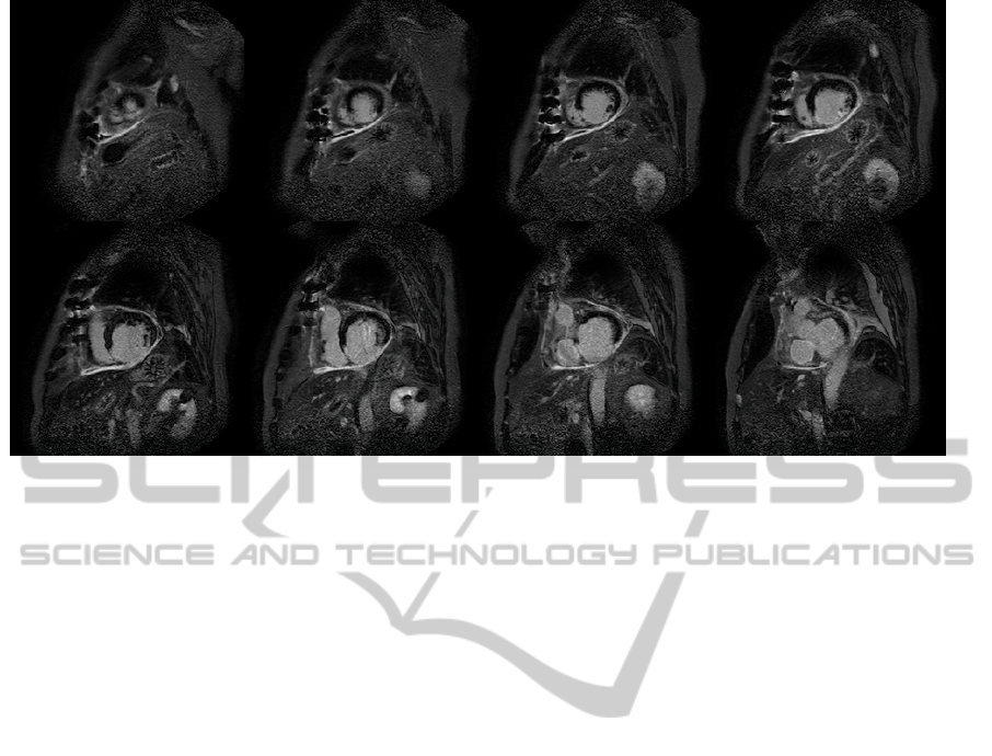
Figure 1: LGE-MRI slices of a patient with myocardial scar. Approximately at the middle of each slice there is an almost

circular and brighter area which is the bloodpool of the heart. The myocardial muscle tissue surrounding the bloodpool is

dark, and in a healthy subject it would have the appearance of a ring. In LGE-MRI, however, scarred tissue with reduced blood

ﬂow will appear brighter. Here we see that the myocardial muscle is partly as bright as the bloodpool because of infarction

scar. The inner border of the myocardial muscle (the dark and partly bright ring) is the endocardium border. The outer border

of the myocardial muscle is called the epicardium border.

1.2 Relation to Prior Work

There have been attempts to solve the problem of au-

tomatic segmentation reported in the literature. Some

methods require manual input in the form of land-

marks or cropping of region of interest, etc (de Brui-

jne and Nielsen, 2004; Spreeuwers and Breeuwer,

2003; Heiberg et al., 2010). Others make use of ad-

ditional data as the corresponding cine MR (ODon-

nell et al., 2003; Ciofolo et al., 2008; Wei et al., 2011;

Wei et al., 2013), or a combination of cine images and

some manual input (Dikici et al., 2004). However, the

use cine-MR requires a suitable registration onto the

LGE-CMR dataset, and this includes potential difﬁ-

culties since patients position and holding of breath

can introduce misalignments.

In our work all results are based solely on the

LGE-CMR images. We presented a method for au-

tomatically ﬁnding the heart center in (Engan et al.,

2013b) and segmentation of the epicardium (Engan

et al., 2013a) with some early results. In this paper we

have continued this work and are presenting a method

for automatic segmentation of the endocardium. A

priori knowledge of typical heart size and shape is

used as the input, and an a posteriori probability map

is made iteratively. The ﬁnal segmentation is based

on the a posteriori probability maps, and information

from all slices are taken into account. Recent work by

Alb

a et.al. (Alba et al., 2012), (Alba et al., 2013) is

also based on the LE-CMR images alone without the

need of cine MR sequences and corresponding reg-

istration. The 3D information and a conical model

are utilized to detect initialization, somewhat similar

to the way we ﬁnd the heart center in (Engan et al.,

2013b).

2 PROPOSED METHOD

The proposed method for segmentation of the my-

ocardium is based on an iterative algorithm ﬁnding

an a posteriori probability map, where the probability

map can be interpreted as the probability of a speciﬁc

pixel belonging to the myocardium. A block diagram

of the complete system can be seen in Figure 2. The

system starts by an algorithm for automatically ﬁnd-

ing the heart center from the whole LGE-CMR slices

with no pre-cropping (block 1). This part will not be

described here, but we proposed two algorithms for

solving this problem in (Engan et al., 2013b). Using

the heart center (HC) as input, an a priori model is

made (block 2), and by using the iterative algorithm

(block 3), an a posteriori probability model is found.

This a posteriori model gives a good foundation for

the last segmentation step of both the epicardium and

the endocardium. The iterative algorithm of block 3 is

important in the context of this paper, thus described

BIOIMAGING2015-InternationalConferenceonBioimaging

here. However a version of this was presented in (En-

gan et al., 2013a) together with some early results on

segmenting the epicardium (block 4). The main fo-

cus of this paper is block 5, segmentation of the en-

docardium. The algorithm is shown and some results

comparing with watershed segmentation of the blood-

pool is presented in the results section.

In the following, let f

(x), i = 1 . .. N

slice

represent

the left ventricle short axis LGE-CMR images of a

patient. x = [x

row

column

]

is the pixel position, and i

represents the slice number.

2.1 Probability Map

The LGE-CMR images are hard to segment because

the scars are bright, whereas the muscle is dark, the

scars have similar intensity levels as the blood pool in-

side the endocardium border, and the edges are some

places non-exsisting. The reason why an expert cardi-

ologist is capable of segmenting the images manually

is that the cardiologist will automatically use prior in-

formation of typical shapes and sizes of a heart. In

the left ventricle short axis view the myocardium will

more or less have the shape of a ring, and this infor-

mation has to be utilized.

We propose to use a rough a priori model of the

myocardium around the heart center for each slice im-

posed as a gaussian in the polar domain with the heart

center as the origin for all angles. µ of the gaussian

prior will correspond to the approximated radius at

the middle of the myocardium for that slice, and is

varied with the slice number. Typical values are found

from a training set, but a large variance is used in the

gaussian prior to make the a priori model robust. Af-

ter mapping to cartesian coordinates and scaling all

pixels to be within [0, 1], this gives an a priori proba-

bility map, where the probability is seen as the prob-

ability for being a pixel in the myocardium.

Using the a priori probability model as input, we

propose an iterative approach to reﬁne the model and

make an a posteriori probability map for the my-

ocardium. At each iteration the probability model

is combined with the inverse of the original (prepro-

cessed) slices, a low pass ﬁltering over the neighbor-

ing slices is performed, and the output is a new prob-

ability model. The inverse of the original is used be-

cause the myocardial muscle we want to segment ap-

pears dark in the images, and thus appears bright with

high values in the inverse. The algorithm is depicted

in Algorithm 1, and a brief explanation follows.

In line (3) of Algorithm 1, a morphological noise

removal of the original slices, f

is conducted using

the morphological center, as deﬁned in (Soille, 2003),

and the structuring element B

as a square of size

Algorithm 1: Iterative probability map algo-

rithm.

Data: CMR images f

(x) ∈ R

N×M

, Prior prob.

map p

(x) ∈ R

N×M

i = 1, . . . N

slice

Result: Posteriori prob. map,

post

(x) ∈ R

N×M

, i = 1, . . . N

slice

1 initialization: k

f inal

;

2 for i ← 1 to N

slice

3 f

prep

(x) ← β

( f

) ;

4 f

inv

(x) =scale(ones(N, M) − f

prep

(x));

5 end

6 for k ← 0 to k

f inal

− 1 do

7 f

temp

(x) = p

(x) × f

inv

(x);

8 f

temp

(x) ← LP f iltZ( f

temp

(x)) ;

9 p

k+1

(x) ← scale( f

temp

(x));

10 end

11 p

nof

(x) = p

(x) × ( f

inv

(x))

f inal

;

12 p

post

(x) =

scale(w

f inal

(x) + (1 − w

nof

(x));

13 return(p

post

) ;

3 × 3 pixels. The noise removal results in a prepro-

cessed slice, f

prep

(x), and the inverse of the prepro-

cessed slice is found in line (4) as f

inv

(x). The main it-

eration is done in line 6-10, using the previous proba-

bility map, f

temp

(x) = p

(x)× f

inv

(x), Low Pass (LP)

ﬁltering over the slices, LP f iltZ( f

temp

(x)), and sub-

sequenty ﬁnding a new probability map, p

k+1

(x) by

scaling the result of the ﬁltering. Another map is

found without ﬁltering over the slices, p

nof

(x), di-

rectly without any iterations as (line 11): p

nof

(x) =

(x) × ( f

inv

(x))

f inal

. The ﬁnal probability model is

a scaled and weighted sum (line 12) between p

f inal

(x)

and p

nof

(x). A × B denotes the Hademard product.

In Figure 3 an example patient is depicted. Top

two rows show the a priori probability map, middle

rows show the a posteriori probability map, and last

two rows shows the original images for this patient.

2.2 Segmentation

The a posteriori probability map looks promising,

but still the segmentation is challenging. The scarred

areas might appear quite dark in the probability im-

ages, thus the probability values can differ signif-

icantly at different angles. Consequently, a global

thresholding technique will not work, regardless of

the chosen threshold. The heart center at each slice,

is an important input, and from the heart cen-

ter the probability values at all radii are evaluated at

different angles, θ ∈ [0, 2π] for both epicardium and

SegmentationofLGEnhancedCardiacMRI

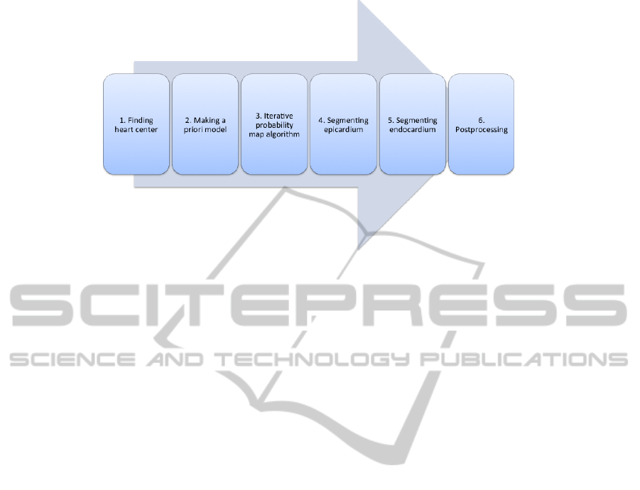
Figure 2: Block diagram of the segmentation scheme.

endocardium segmentation. Since we know that the

endocardium borders lie within the epicardium bor-

ders, we start by ﬁnding the epicardium mask and use

that as a input for the endocardium segmentation.

The algorithm for segmenting the epicardium was

presented and explained in (Engan et al., 2013a) and

will not be repeated here. In short, the epicardium

segmentation algorithm uses the a posteriori proba-

bility map as well as the heart centers as input. A mor-

phological closed-hole preprocessing of the probabil-

ity map is done prior to a Otsu’s multilevel threshold-

ing. Using the heart center position in each slice, HC

as origin, the values after the multilevel thresholding

are interpreted in polar coordinates giving R

(θ, r),

where θ is the angle and r the radius. The partial

derivative of R

(θ, r) with respect to r is found for all

θ, D

(θ, r), and the ﬁrst negative value of the deriva-

tive (smallest radius) is marked as a candidate epi-

cardium border point, R

epi

(θ), for each θ. Some ﬁnal

steps are dealing with angles with missing candidate

points by looking at neighboring angles and slices.

The proposed segmentation of the endocardium

is also based on the a posteriori probability map,

post

(x) ∈ R

N×M

, i = 1, . . . N

slice

. The segmentation

of the epicardium is executed ﬁrst, and a resulting epi-

cardium mask, Mask

epicard

(x), is used as additional

information since the endocardium must lie inside

the epicardium. A pseudocode of the algorithms for

endocardium segmentation based on the probability

maps is seen in Algorithm 2, and an explanation fol-

lows:

A multilevel version of Otsu’s method (Otsu,

1979) is used for non uniformly quantizing of p

post

(x)

into L levels: f

(x) = Quant

nonuni

post

(x), L) (line

3). In line 4, the Hademar product between the quan-

tized probability images and the epicardium mask sets

qepi

(x) to zero outside the epicardium.

Thereafter a conversion to polar coordinates with

the heart center as the origin is performed giving

(θ, r). For each angle a candidate endocardium

point is looked for as seen in line 7.

Let R

(θ, 0) denote the value at the HC (heart cen-

ter) point. If there exist points in R

(θ, r) with value

(θ, r

) > R

(θ, 0) + 1, and r

is the point closest

to HC, then R

endo

(θ) = r

. If not, there might exist

points with value R

(θ, r

) > R

(θ, 0), and let r

the point closest to HC, then R

endo

(θ) = r

. If nei-

ther of these points exists there are no candidate point

for that speciﬁc angle at slice i.

If an angle, θ

, is without candidate points for

slice i, the other slices are checked to see if there ex-

ist any candidate points for θ

(line 13-15). If any

of the other slices have candidate points for θ

, the

one corresponding to the slice closest to slice i is

chosen for slice i as well. If there are no candidate

points for θ

for any slices, the smallest ∆

to an an-

gle with a candidate point is found within slice i, ap-

proximating the candidate point for θ

using the same

endo

(θ

+ ∆

) (line 16-18). Finally the convex hull

of all candidate points is found as the endocardium

mask, Mask

endocard

(x)) (line 22).

2.3 Postprocessing

The endocardium mask Mask

endocard

(x) over the

slices i = 1, . . . N

slice

are compared. If there are

segments that are only present in Mask

endocard

(x)

it is considered a mistake, and removed from

Mask

endocard

(x). If there are segments present in

all slices except Mask

endocard

(x), this segment is

added to Mask

endocard

(x). After ﬁnding the endo-

cardium mask, the perimeter is calculated. Thereafter

BIOIMAGING2015-InternationalConferenceonBioimaging

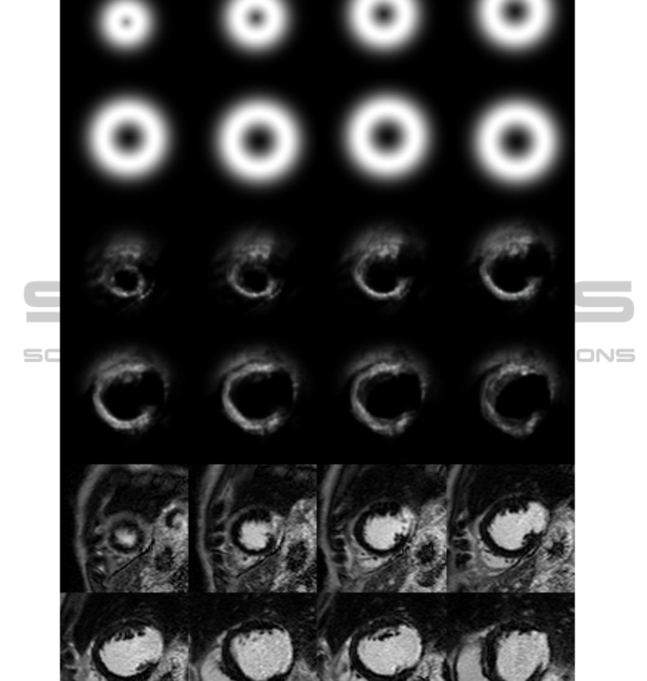
Figure 3: Top two rows, a priori probability map, second two rows, a posteriori probability map after 8 iterations, last two

rows, original images.

a Fourier Descriptor (FD) (Impedovo et al., 1978) of

this perimeter is found. The FD is lowpass ﬁltered

resulting in a smoother perimeter and a new mask.

3 EXPERIMENTS AND RESULTS

Segmentation experiments are performed on the set of

54 patients, 395 images. Different number of levels,

L, in the multilevel version of Otsus method in Algo-

rithm 2 were tested in preliminary experiments. L=4

seemed to preform best and is used in the experiments

presented here. The number of iterations of the itera-

tive probability map scheme was set to 8. Results are

presented as Dice (Dice, 1945) and Jaccard (Jaccard,

1912) indices.

The mean and standard deviation of the resulting

Dice and Jaccard indices of the endocardium segmen-

SegmentationofLGEnhancedCardiacMRI

Algorithm 2: Radial Segmentation of endo-

cardium.

Data: CMR images f

(x) ∈ R

N×M

, Posteriori

prob. map,

post

(x) ∈ R

N×M

, i = 1, . . . N

slice

, heart

center coordinates HC

, Mask

epicard

(x) ;

Result: Mask

endocard

(x)

1 initialization: R

endo

(θ) = 0, θ ∈ [0, 2π];

2 for i = 1 to N

slice

3 f

(x) = Quant

nonuni

post

(x), L) ;

4 f

qepi

(x) = f

(x) × Mask

epicard

(x) ;

5 for θ = 0 to 2π do

6 R

(θ, r) = cart2poly( f

qepi

(x), θ, HC

) ;

7 R

endo

(θ) = argmax(argmin

(θ, r) >

(θ, 0) + 1)], argmin

(θ, r) >

(θ, 0)]) ;

8 end

9 R

endo

(θ) ← smooth(R

endo

(θ)) ;

10 end

11 for i = 1 to N

slice

12 for θ = 0 to 2π do

13 if R

endo

(θ) = 0 then

14 R

endo

(θ) ← mean(R

endo

(θ) 6= 0)

15 end

16 if R

endo

(θ) = 0 then

17 R

endo

(θ) ←

min

|∆

endo

(θ − ∆

) 6= 0)

18 end

19 x

= poly2cart(R

endo

(θ)) ;

20 f

) = 1;

21 end

22 Mask

endocard

(x) = ConvexHull( f

(x));

23 end

24 return(Mask

endocard

(x)) ;

tation are seen in Table 2 where the automatic method

for ﬁnding the heart center is used. In Table 3 the re-

sults from the same experiments, but using the true

heart center as input, are shown. In Table 1 the mean

and standard deviation of Dice index of both the en-

docardium and epicardium over all the images are

Table 1: Results for segmentation of endocardium and epi-

cardium. Dice index, averaged over 395 images. Standard

deviation in parentheses.

Endocard Epicard

Dice Dice

True HC 0.87 (0.040) 0.90 (0.034)

Automatic HC 0.85 (0.048) 0.88 (0.046)

shown comparing results using the true heart center

with the automatically found heart center. Two slices

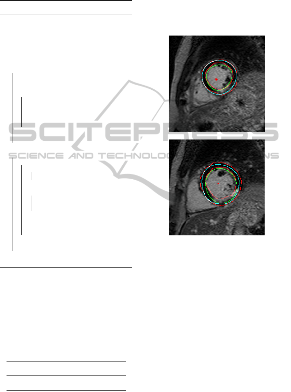
of an example patients are seen in detail in Figure 4

for illustration.

Figure 4: Segmentation results from two slices of an exam-

ple patient. manual marking performed by cardiologist in

red, automatically found heart center marked as red stars,

epicaridum contours in cyan, and endocardium contours in

green. The top slice shows well performing segmentation.

In the bottom slice the epicardium is segmented well, but

the segmentation of the endocardium fails to include the

scar in the myocardium

3.1 Comparison with Watershed

Segmentation

To compare the proposed method with a classi-

cal and successful segmentation algorithm, we have

compared with marker controlled watershed (Meyer,

1994; Soille, 2003) using different gradient images,

and different markers.

Watershed segmentation was conducted using a

morphological gradient on the CMR-images after

some noise reduction was performed by using the

BIOIMAGING2015-InternationalConferenceonBioimaging

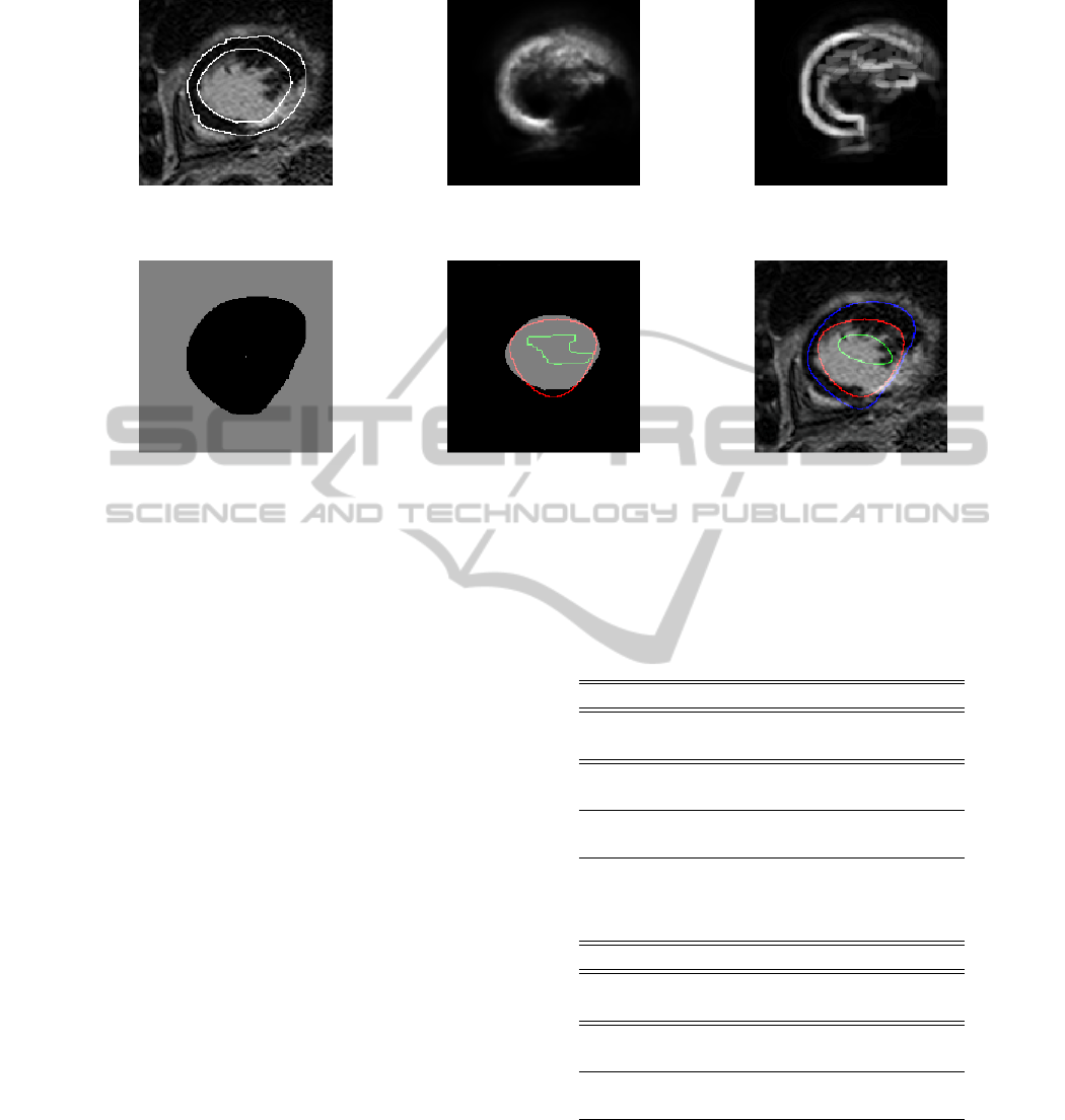
Figure 5: Segmentation results from one slice of an example patient. First row, left to right: Original image with manual

markings, a posteriori probability map, gradient from a posteriori probability map. Second row, left to right: epicardium mask

from automatic method used as external marker, true endocardium mask with proposed method in red and WS

PMGepi

in green,

original image with overlaid contours of epicardium (blue) endocardium (proposed method, red) and WS

PMGepi

(green) after

post processing.

morphological center algorithm (Soille, 2003). The

corresponding results are named WS

when the

external marker was the edge of the cropped im-

age, where the cropping was done automatically us-

ing the hear center as input, and WS

MGepi

when the

external marker is deﬁned by the epicardium mask,

Mask

epicard

(x). The latter is done since the endo-

cardium border cannot cross the (true) epicardium

border.

Watershed segmentation using the a posteriori

probability map images as input to ﬁnd the morpho-

logical gradient images was also executed. The re-

sults are named WS

PMG

when the external marker

is the edge of the cropped image, and WS

PMGepi

when the external marker is deﬁned by the epicardium

mask, Mask

epicard

(x). Two different internal marker

are tested; the heart center from our proposed au-

tomatic method using the circular Hough Transform

(CHT), see Table 2, and the true heart center, see Ta-

ble 3.

Results from some slices of an example patient are

depicted in Figure 6. For this example patient we can

see that the proposed method performs better than the

depicted WS

MGepi

, since the latter includes more of

the scar in the bloodpool. One slice of another exam-

ple patient is depicted in Figure 5 at different stages

together with the result of the proposed method as

well as WS

PMGepi

. In this example the WS

PMGepi

Table 2: Jaccard and Dice index, averaged over 395 images.

Standard deviation in parentheses. Heart center from auto-

matic method.

Endocard seg. Dice Jaccard

Prop.method 0.85 (0.048) 0.74 (0.070)

0.80 (0.075) 0.68 (0.099)

MGepi

0.83 (0.060) 0.71 (0.084)

PMG

0.78 (0.050) 0.65 (0.068)

PMGepi

0.79 (0.066) 0.65 (0.086)

Table 3: Jaccard and Dice index averaged over 395 images.

True heart center (HC) as input.

Endocard seg. Dice Jaccard

Prop.method 0.87 (0.040) 0.77 (0.062)

0.80 (0.075) 0.68 (0.099)

MGepi

0.84 (0.055) 0.72 (0.080)

PMG

0.80 (0.055) 0.67 (0.075)

PMGepi

0.81 (0.068) 0.69 (0.088)

fails completely whereas the proposed method per-

forms quite well.

SegmentationofLGEnhancedCardiacMRI

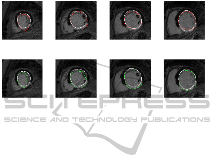
Figure 6: Segmentation results from some slices of an example patient. First row, white is manual marking, red is result from

proposed method, dice index of this patient is 0.90. Second row, white is manual marking, green is WS

MGepi

, Dice index of

this patient is 0.84.

4 CONCLUSION

The presented method for segmentation of endo-

cardium in LGE-CMR completes a larger system

for automatic segmentation of the myocardium in

LGE-CMR. The proposed system is based on us-

ing some prior information about LGE-CMR images:

the bloodpool and the myocardial muscle is approx-

imately circular and this is used when constructing

an a priori probability map. The 3D information is

utilized both ﬁnding the heart center and when pro-

ducing the a posteriori probability map. The CMR

images are not true 3D in the sense that the resolution

in the z-direction (i.e. between slices) is much coarser

then the resolution within a slice.

All experiments are conducted on a dataset of 54

patients, all with myocardial infarctions. Twenty of

these patients are patients implanted with ICD (CMR

images recorded prior to implantation), and these

patients have severe scars, and sometimes enlarged

hearts, making the segmentation even more challeng-

ing.

Results on the endocardium segmentation using

the proposed method was compared to results using

watershed with different gradients and different ex-

ternal markers. The mean Dice and Jaccard of the

proposed fully automatic method are 0.85 and 0.74

respectively. Using the true heart center as input im-

proves the Dice index to 0.87 and the Jaccard index

to 0.77 showing the potential of the latter part of the

proposed system. Watershed gave the corresponding

results 0.8 and 0.68. Using the epicardium segments

from the proposed method as the external marker im-

proved the watershed results, were the best results

gave Dice index 0.83 and Jaccard index 0.71. The

reported results in (Alba et al., 2012) are very good

(Mean Dice index of 0.81 for the myocardial mus-

cle), but on a limited dataset of LGE-CMR images

(20 patients). In future work we will strive to do a fair

comparison of our method with (Alba et al., 2013) .

REFERENCES

Alba, X., i Ventura, R. F., Lekadir, K., and Frangi, A.

(2012). Conical deformable model for myocardial

segmentation in late-enhanced MRI. In Proceed-

ings of IEEE International Symposium on Biomedical

Imaging (ISBI. 10.1109/ISBI.2012.6235536.

Alba, X., i Ventura, R. F., Lekadir, K., Tobon-Gomez,

C., Hoogendoorn, C., and Frangi, A. (2013). Au-

tomatic cardiac lv segmentation in MRI using mod-

iﬁed graph cuts with smoothness and interslice con-

straints. Magnetic Resonance in Medicine. doi:

10.1002/mrm.25079.

Ciofolo, C., Fradkin, M., Mory, B., Hautvast, G., and

Breeuwer, M. (2008). Automatic myocardium seg-

mentation in late-enhancement MRI. In Proceed-

ings of IEEE International Symposium on Biomedical

Imaging (ISBI).

de Bruijne, M. and Nielsen, M. (2004). Shape particle ﬁl-

tering for image segmentation. In Proc. of MICCAI,

volume 3216, pages 168–175.

Dice, L. R. (1945). Measures of the amount of ecologic

BIOIMAGING2015-InternationalConferenceonBioimaging

association between species. Ecology, 26(3):297–302.

doi:10.2307/1932409.

Dikici, E., ODonnell, T., Setser, R., and White, R. (2004).

Quantiﬁcation of delayed enhancement MR images.

In Proceedings of the International Conference on

Medical Image Computing and Computer-Assisted In-

tervention, pages 250–257.

Engan, K., Naranjo, V., Eftestøl, T., Ørn, S., and Woie, L.

(2013a). Automatic segmentation of the epicardium

in late gadolinium enhanced cardiac MR images. In

Proc. of Comp. in Cardiology 2013, Zaragoza, Spain.

Engan, K., Naranjo, V., Eftestøl, T., Woie, L., Schuchter,

A., and Ørn, S. (2013b). Automatic detection of heart

center in late gadolinium enhanced MRI. In Proceed-

ings of MEDICON 2013, Sevilla, Spain.

Heiberg, E., Sjgren, J., Ugander, M., Carlsson, M., Eng-

blom, H., and Arheden, H. (2010). Design and valida-

tion of segment a freely available software for cardio-

vascular image analysis. In BMC Medical Imaging,

volume 10:1.

Impedovo, S., Marangelli, B., and Fanelli, A. M. (1978). A

fourier descriptor set for recognizing nonstylized nu-

merals. IEEE Trans. Sys., Man., Cyber, 8(8):640–645.

doi: 10.1109/TSMC.1978.4310042.

Jaccard, P. (1912). The distribution of the ﬂora in the alpine

zone. New Phytologist, (11):37–50.

Meyer, F. (1994). Topographic distance and watershed

lines. Signal Processing, 38:113–125.

ODonnell, T., Xu, N., Setser, R., and White, R. (2003).

Semi-automatic segmentation of nonviable cardiac

tissue using cine and delayed enhancement magnetic

resonance images. In Proceedings of SPIE 2003, vol-

ume 5031, page 242.

Otsu, N. (1979). A threshold selection method from gray-

level histograms. IEEE Trans. Sys., Man., Cyber,

9(1):62–66. doi:10.1109/TSMC.1979.4310076.

Soille, P. (2003). Morphological Image Analysis. Springer-

Verlag, Berlin Heidelberg, Germany, 2 edition.

Spreeuwers, L. and Breeuwer, M. (2003). Detection of

left ventricular and epi- and endocardial borders using

coupled active contours. In Proc. Comput. Assisted

Radiol. Surg., page 11471152.

Thygesen, K., Alpert, J., White, H., and et.al. (2007). Uni-

versal deﬁnition of myocardial infarction. European

Heart Journal, 28(20):2525–2538.

Wei, D., Sun, Y., Chai, P., Low, A., and Ong, S. (2011).

Myocardial segmentation of late gadolinium enhanced

mr images by propagation of contours from cine mr

images. Med Image Comput Comput Assist Interv,

14:428–35.

Wei, D., Sun, Y., Ong, S., Chai, P., Teo, L. I., and Low,

A. F. (2013). Three-dimensional segmentation of the

left ventricle in late gadolinium enhanced mr images

of chronic infarction combining long- and short-axis

information. Medical Image Analysis, 17(6):685–697.

doi:10.1016/j.media.2013.03.001.

SegmentationofLGEnhancedCardiacMRI