On Selecting Useful Unlabeled Data Using Multi-view Learning
Techniques
∗
Thanh-Binh Le and Sang-Woon Kim
Department of Computer Engineering, Myongji University, Yongin, 449-728 Korea
Keywords:
Semi-supervised Learning, Selecting Unlabeled Data, Multi-view Learning Techniques.
Abstract:
In a semi-supervised learning approach, using a selection strategy, strongly discriminative examples are first
selected from unlabeled data and then, together with labeled data, utilized for training a (supervised) classifier.
This paper investigates a new selection strategy for the case when the data are composed of different multiple
views: first, multiple views of the data are derived independently; second, each of the views are used for mea-
suring corresponding confidences with which examples to be selected are evaluated; third, all the confidence
levels measured from the multiple views are used as a weighted average for deriving a target confidence; this
selecting-and-training is repeated for a predefined number of iterations. The experimental results, obtained
using synthetic and real-life benchmark data, demonstrate that the proposed mechanism can compensate for
the shortcomings of the traditional strategies. In particular, the results demonstrate that when the data is ap-
propriately decomposed into multiple views, the strategy can achieve further improved results in terms of the
classification accuracy.
1 INTRODUCTION
In semi-supervised learning (SSL) approaches (Zhu,
X. and Goldberg, A. B., 2009), a large amount of un-
labeled data (U), together with labeled data (L), is
used to build better classifiers. However, it is also
well known that using U is not always helpful for
SSL algorithms. In particular, it is not guaranteed that
addingU to the training data (T), i.e. T = L∪U, leads
to a situation in which the classification performance
can be improved. Therefore, in order to select a small
amount of useful unlabeled data, various sampling
(and selecting) techniques have been proposed in
the literature, including the self-training (Yarowsky,
1995), co-training (Blum, A. and Mitchell, T., 1998),
confidence-based approaches (Le, T. -B. and Kim, S. -
W., 2014; Mallapragada, P. K. et al., 2009), and other
approaches used in active learning (AL) algorithms
(Dagan, I. and Engelson, S. P., 1995; Reitmaier, T.
and Sick, B., 2013). However, in AL, selected in-
stances are useful when they are labeled, thus it is re-
quired to query their true class label from a human
annotator. From this point of view, the approaches for
SSL and AL algorithms are different.
∗
This work was supported by the National Research
Foundation of Korea funded by the Korean Government
(NRF-2012R1A1A2041661).
In SemiBoost (Mallapragada, P. K. et al., 2009),
for example, the confidence level of all x
i
∈ U exam-
ples is first computed based on the prediction made
by an ensemble classifier and the similarity among the
examples of L∪U. Then, a few examples with higher
confidence are selected to retrain the ensemble classi-
fier together with L. This selecting-and-training step
is repeated for a predefined number of iterations or
until a termination criterion is met. More specifically,
the confidence level is computed using two quantities,
i.e. p
i
(= p(x
i
)) and q
i
(= q(x
i
)), which are measured
using the pairwise similarity between x
i
∈ U and other
L and U examples. However, when x
i
is near the
boundary between two classes, the value is computed
using U only, without referring to L. Consequently,
the value might be inappropriate for selecting useful
examples.
In order to address this problem, a modified cri-
terion that minimizes the errors in estimating the la-
bels of U examples has been considered (Le, T. -B.
and Kim, S. -W., 2014). In the modified criterion, for
x
i
∈ U that are near the boundary between the posi-
tive class of L (L
+
) and the negative class of L (L
−
),
the confidence levels (and predicted pseudo labels)
are measured using estimates of the class-conditional
probabilities (P
E
) as well as the quantities of p
i
and
q
i
. However, sometimes the modified criterion devel-
157
Le T. and Kim S..
On Selecting Useful Unlabeled Data Using Multi-view Learning Techniques.
DOI: 10.5220/0005171301570164
In Proceedings of the International Conference on Pattern Recognition Applications and Methods (ICPRAM-2015), pages 157-164
ISBN: 978-989-758-076-5
Copyright
c
 2015 SCITEPRESS (Science and Technology Publications, Lda.)

ops a weakness. In general, the reason for this can
be explained as follows: for the modified criterion,
the confidence level, which is denoted using a ρ1(x
i
)
symbol, is determined with four terms of the L
+
, L
−
,
U concerned terms and P
E
included as a certainty
level. Thus, when L
−
and L
+
terms are similar, as a
consequence ρ1(x
i
) depends on U and P
E
terms only.
Therefore, when L examples are highly overlapped,
P
E
cannot work well and in turn, ρ1(x
i
), which com-
pletely depends on the deeply overlapped U exam-
ples, cannot work as well. In order to address this is-
sue, a selection strategy utilizing multi-view learning
techniques is investigated in this paper.
Currently, multi-view data is common in a wide
variety of applications (Kumar, A. and Daume III, H.,
2011). This is the motivation for an approach of se-
lecting useful unlabeled data based on the multi-view
setting in this paper: first, a partition of the attributes
of the data is found using either a similarity mea-
sure between pair-wise examples or a feature selec-
tion function; corresponding views are derived inde-
pendently; each of the views is used for measuring
its confidence; finally, all the confidences measured
from the views are used as a weighted average for de-
riving a target confidence. The central idea to the pro-
posed strategy is that the confidence obtained from
one view could be helpful for deriving another confi-
dence from another view. The strategy is empirically
compared with some traditional methods using syn-
thetic and real-world data.
The main contribution of this paper is the demon-
stration that the classification accuracy of the super-
vised / semi-supervised classifiers can be improved
using the multi-view based selection strategy. In par-
ticular, it is demonstrated that when the data is suf-
ficiently decomposed into multiple views, the classi-
fication accuracy is significantly improved. The re-
mainder of the paper is organized as follows: in Sec-
tion 2, a brief introduction to the selection criteria
used in SemiBoost and its modified version is pro-
vided; in Section 3, a method of utilizing the multi-
view based criterion is presented; in Section 4, an il-
lustrative example for comparing the selection criteria
and the experimental results obtained using the real-
life datasets are presented; in Section 5, the conclud-
ing remarks are presented.
2 RELATED WORK
2.1 Sampling in SemiBoost
The goal of SemiBoost is to iteratively improve the
performance of a supervised learning algorithm (A )
by using U and pairwise similarity. In order to follow
the boosting idea, SemiBoost optimizes performance
through minimizing an objectiveloss function defined
as Proposition 2 in (Mallapragada, P. K. et al., 2009)),
where h
i
(= h(x
i
)) is the base classifier learned by A
at the iteration, α is the weight for combining h
i
’s, and
p
i
=
n
l
∑
j=1
S
ul
i, j
e
−2H
i
δ(y
j
,1) +
C
2
n
u
∑
j=1
S
uu
i, j
e
H
j
−H
i
,
q
i
=
n
l
∑
j=1
S
ul
i, j
e
2H
i
δ(y
j
,−1) +
C
2
n
u
∑
j=1
S
uu
i, j
e
H
i
−H
j
.
(1)
Here, H
i
(= H(x
i
)) denotes the final combined
classifier and S denotes the pairwise similarity:
S(i, j) = exp(−kx
i
− x
j
k
2
2
/σ
2
) for all x
i
and x
j
of
the training set, where σ is the scale parameter con-
trolling the spread of the function. In addition, S
lu
(and S
uu
) denotes the n
l
× n
u
(and n
u
× n
u
) subma-
trix of S, where n
l
= |L| and n
u
= |U|. Also, S
ul
and
S
ll
can be defined correspondingly; the constant C,
which is computed using C = |L|/|U| = n
l
/n
u
, is in-
troduced to weight the importance between L and U;
and δ(a,b) = 1 when a = b and 0 otherwise.
The quantities of p
i
and q
i
can be interpreted as
the confidence in classifying x
i
∈ U into a positive
class and negative class, respectively. That is, p
i
and
q
i
can be used to guide the selection of U examples
at each iteration using the confidence measurement
|p
i
− q
i
|, as well as to assign the pseudo class label
sign(p
i
− q
i
). From (1), a selection criterion can be
formulated as follows:
p
i
− q
i
=


e
−2H
i
∑
x
j
∈L
+
S
ul
i, j


−


e
2H
i
∑
x
j
∈L
−
S
ul
i, j


+
C
2
∑
x
j
∈U
S
uu
i, j
(e
H
j
−H
i
− e
H
i
−H
j
)
!
,
(2)
where L
+
≡ {(x
i
,y
i
)|y
i
= +1,i = 1, ··· , n
+
l
} and L
−
≡
{(x
i
,y
i
)|y
i
= −1, i = 1,·· · ,n
−
l
} are the L examples in
class {+1} and class {−1}, respectively. In (2), by
substituting the three corresponding summations with
X
+
i
, X
−
i
, and X
u
i
symbols, the criterion can be repre-
sented as: p
i
− q
i
= X
+
i
− X
−
i
+ X
u
i
.
However, providing more data is not always ben-
eficial. If the value obtained using the third term in
(2) is very large or X
+
i
is nearly equal to X
−
i
, (2) will
generate some erroneous data. In that case, the mean-
ing achieved using the confidence of X
+
i
− X
−
i
may
be lost and the estimation for x
i
will depend on the U
examples. That is, the L examples do not affect the
estimation of x
i
label; therefore, the estimated label is
unsafe and untrustworthy.
ICPRAM2015-InternationalConferenceonPatternRecognitionApplicationsandMethods
158

2.2 Modified Criterion
As mentioned previously, using p
i
and q
i
can lead to
incorrect decisions in the selection and labeling steps;
this is particularly common when the summation of
the similarity measurement from x
i
∈ U to x
j
∈ L is
too weak.
In order to avoid this, the criterion of (2) can be
improved through balancing the three terms in (2), i.e.
X
+
i
, X
−
i
, and X
u
i
. Using the probability estimates as
a penalty cost, the criterion of (2) can be modified as
follows:
ρ1(x
i
) =


X
+
i
− X
−
i
+ X
u
i
− (1− P
E
(x
i
))


, (3)
where P
E
(x
i
) denotes the class posterior probability of
instance of x
i
(i.e. a certainty level and 1−P
E
(x
i
) cor-
responds to the percentage of mistakes when labeling
x
i
.
However, it should be noted that sometimes us-
ing (3) leads to a problematic situation. When all
x
i
∈ U are well-separated and correctly distributed,
P
E
(x
i
) can be measured successfully and, in turn, the
criterion of (3) works well. However, for the case
where the L∪U examples are composed of (different)
multiple views (i.e., feature vectors of the data consist
of different attribute subsets) and, especially, they are
near the boundary between two classes, ρ1(x
i
) may
not work for selecting good examples from U. Gen-
erally, the reason for this can be explained as follows.
ρ1(x
i
) is computed from distance measurements be-
tween pair-wise examples of L∪U. Under X
+
i
≈ X
−
i
,
computation of ρ1(x
i
) is completely determined from
X
u
i
and P
E
(x
i
). As a consequence, deeply overlapped
distribution of U examples leads to a problematic sit-
uation, where P
E
(x
i
) cannot work well and, in turn,
ρ1 cannot work as well.
3 PROPOSED METHOD
3.1 Newly Modified Criterion
Assume that a data set X = {x
1
,·· · ,x
n
}, x
i
∈ R
d
consists of two views with their respective feature
partitions: X
1
= {x
11
,·· · ,x
1n
}, x
1i
∈ R
d
1
, and X
2
=
{x
21
,·· · ,x
2n
}, x
2i
∈ R
d
2
, where d = d
1
+ d
2
. That is,
they are two attribute subsets describing the data X.
In the multi-view learning (de Sa, V., 1994), two clas-
sifiers, h
1
and h
2
, are trained using L, both on their
respective views; they operate on different views of
an example: h
1
is based on L
1
, h
2
is based on L
2
.
The two classifiers are then evaluated using U; af-
ter classifying the remaining data of U, with h
1
and
h
2
separately, the examples (i.e., U
s
) on which it is
the most confident are removed from U and added
to L for the next iteration, i.e. {(x
i
,h
1
(x
i
))} to L
2
and {(x
i
,h
2
(x
i
))} to L
1
. Both classifiers are now re-
trained on the expanded L
1
and L
2
sets and the proce-
dure is repeated until some stopping criteria is met.
In order to select useful unlabeled data, the multi-
view learning technique can be utilized as follows:
first, each of the related data sets is divided into two
different views (i.e., L
k
,U
k
, and S
k
, where k = 1,2) us-
ing a feature selection scheme; next, as in (2), for all
x
ki
∈ U
k
, after designing h
k
per view, the confidence
levels of x
ki
, using |p
ki
− q
ki
|, and the classification
error rates ε(h
k
), using all L
j
, (j 6= k), are computed;
finally, for all x
i
∈ U, using ε(h
k
) as a weight, its con-
fidence level (which is newly denoted using a ρ2(x
i
)
symbol) can be measured as follows:
ρ2(x
i
) =
K
∑
k=1
1
ε (h
k
)
|p
ki
− q
ki
|. (4)
Using (4) as a selection criterion, a sampling func-
tion, named Multi-view Sampling, can be summa-
rized as follows.
Algorithm 1: Multi-view Sampling.
Input: Labeled data (L), unlabeled data (U), view #
of attributes (K = 2), and α (% of selected U over U).
Output: Selected unlabeled data (U
s
).
Procedure: Perform the following steps.
1. Decompose L ∈ R
d
into L
k
, (k = 1,··· ,K), views
first (refer to (1)), where L
k
∈ R
d
k
and d =
∑
K
k=1
d
k
; then, train a classifier (h
k
) per view us-
ing corresponding data L
k
.
2. First, compute a mapping function (w
k
) to trans-
form L to L
k
, i.e. L
k
← L · w
k
; second, using w
k
,
compute U
k
← U · w
k
; third, compute the error
rates, ε(h
k
), using all L
j
, (j 6= k).
3. For all x
ki
∈ U
k
, first, compute confidence levels
(ρ
ki
) per view using p
i
, q
i
, and h
k
; then, average
the levels as ρ2
i
←
∑
K
k=1
1
ε(h
k
)
ρ
ki
, and sort them in
a decreasing order on key {|ρ2
i
|}.
4. Choose U
s
from top α(%) of U and estimate pre-
dicted labels of x
j
∈ U
s
using sign(ρ2
j
).
End Algorithm
3.2 Proposed Algorithm
The proposed learning algorithm initially predicts the
labels of all U examples using a classifier (SVM, for
example) trained with L only. After initializing the
related parameters, e.g. the kernel function and its
OnSelectingUsefulUnlabeledDataUsingMulti-viewLearningTechniques
159

related conditions, the confidence levels of all U ex-
amples (i.e., {|ρ2(x
i
)|}
n
u
i=1
) are calculated using (3).
Then, {|ρ2(x
i
)|}
n
u
i=1
is sorted in descending order. Af-
ter selecting the examples ranked with the highest
confidence levels, adding them to L creates an ex-
panded training set (T).
Finally, the aboveselecting-and-trainingstep is re-
peated, while verifying the training error rates of the
classifier. The repeated regression leads to an im-
proved classification process and, in turn, provides
better prediction of the labels over iterations. Con-
sequently, the best training set, which is composed of
L and U
s
examples (i.e. T = L ∪U
s
), constitutes the
final classifier for the problem.
Based on this brief explanation, a learning algo-
rithm, using the sampling function in Algorithm 1,
is summarized as follows: the labeled and unlabeled
data (L and U), cardinality of U
s
, number of iterations
(e.g. J = 10 and K = 2), and type of kernel function
and its related constants (i.e. C and C
∗
) are given as
input parameters; as outputs, the labels of all data and
the classifier model are obtained.
Algorithm 2: Proposed Learning Algorithm.
Input: Labeled data (L) and unlabeled data (U). Out-
put: Final classifier (H). Method: Initialization: Set
the parameters: J, K, α
(0)
, ∆
(0)
; train a classifier H
(and its error rate ε(H)) using L.
Procedure: Repeat the following steps while increas-
ing j from 1 to J in increments of 1.
1. Obtain U
( j)
s
(and their predicted labels) fromU by
invoking the Multi-view sampling function with
training data T (or L if j = 1), U, K, α
( j)
.
2. Update the training data T using U
( j)
s
, i.e. T ←
L∪U
( j)
s
, and train a classifier (h
j
) (and its classi-
fication error rate, named ε(h
j
)) through T.
3. If ε(h
j
) ≤ ε(H), then keep h
j
as the best classifier,
i.e. H ← h
j
and ε(H) ← ε(h
j
).
4. α
( j+1)
← α
( j)
+ ∆
( j)
.
End Algorithm
4 EXPERIMENTAL RESULTS
4.1 Synthetic Data
First, two 2-dimensional, two-class datasets hav-
ing different Gaussian distributions were generated.
Then, the two 2-dimensional datasets were concate-
nated into a 4-dimensional, two-class dataset.
For the synthetic data, an experiment was con-
ducted as follows: first, two confidence values were
computed for all x
i
∈ U using the three criteria in (2),
(3), and (4), i.e. |p
i
− q
i
|, |ρ1(x
i
)|, and |ρ2(x
i
)|; sec-
ond, a subset of U, i.e. U
s
(the 10% cardinality of U),
was selected referring to the confidence values. These
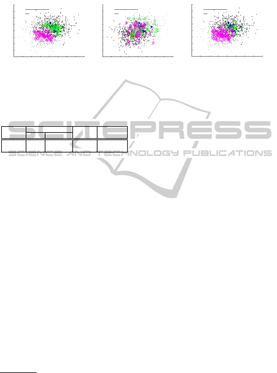
two steps were repeated ten times. Fig. 1 presents a
comparison of three selections obtained with the ex-
periment. Here, the data of (5,5) objects of the two
classes were generated ten times as L. For each gener-
ation of the L data, the data of (500,500) objects were
generated ten times again as U.
From the figure, it can be observed that the ca-
pability of the proposed strategy for selecting use-
ful unlabeled data for discrimination is generally im-
proved. This is clearly demonstrated in the differ-
ences between Fig. 1 (a), (b), and (c) by the number
of selected objects and their geometrical structures.
More specifically, for the boundary regions between
the positive and negative classes in Fig. 1 (a), the
number of the selected objects but overlapped of the
multi-view strategy is smaller than that of the origi-
nal and modified strategies in Fig. 1 (b) and (c). In
contrast, for all the three criteria, there is no object
being selected but overlapped. The selected objects
are all appropriately chosen. From this observation, it
should be noted that the discriminative power of the
multi-view strategy might be better than that of the
original SemiBoost and its modified strategies.
In order to investigate this further, another exper-
iment was conducted on labeling the (selected) unla-
beled data using the three selection strategies. That
is, a verification of the pseudo-labels for each x
i
∈ U
was predicted using the three criteria. The experi-
ment was undertaken as follows: first, as in the above
experiment, a subset (U
s
) was selected from U af-
ter computing the confidence values; second, three
pseudo-labels of all x
i
∈ U
s
were predicted using the
three techniques in (2), (3), and (4), i.e. sign(p
i
− q
i
),
sign(ρ1(x
i
)), and sign(ρ2(x
i
)); third, the predicted
pseudo-labels were compared with their true labels
(y
U
s
∈ {+1,−1}); finally, based on the comparison,
the number of wrongly predicted objects was counted.
Based on this count, in order to clearly compare the
selection criteria, a wrong-prediction rate (ε
Prediction
)
was defined as: ε
Prediction
=
Failed Prediction #
Total Prediction #
.
From Fig. 1 (b), a high value of ε
Prediction
(=
46/100) was obtained using the original criterion. In
contrast, from Fig. 1 (a) and (b), a very small value
of ε
Prediction
(= 0/100) was obtained using the two
modified criteria, i.e. Multi-view and Modified. As
mentioned previously, although the wrong-prediction
rates of the two criteria are the same, among the se-
lected objects, the number of overlapped objects of
ICPRAM2015-InternationalConferenceonPatternRecognitionApplicationsandMethods
160

−1 0 1 2 3 4 5 6 7
−1
0
1
2
3
4
5
6
7
View 2
Feature 3
Feature 4
W rong P redictions
T otal P redictions
=
0
100
=0
(a)
−1 0 1 2 3 4 5 6 7
−1
0
1
2
3
4
5
6
7
View 2
Feature 3
Feature 4
W rong P redictions
T otal P redictions
=
46
100
=0.46
(b)
−1 0 1 2 3 4 5 6 7
−1
0
1
2
3
4
5
6
7
View 2
Feature 3
Feature 4
W rong P redictions
T otal P redictions
=
0
100
=0
(c)
Figure 1: Plots comparing the selected objects with the three selection criteria: (a) the multi-view criterion, (b) the original
criterion, and (c) its modified criterion for the four-dimensional, two-class synthetic data. The results obtained are partially
displayed in [x
3
,x
4
] only (where [x
1
,x
2
]’s are almost the same and omitted here); the objects in the positive and negative
classes are denoted by ‘+’ (in red) and ‘∗’ (in blue) symbols, respectively; the selected objects from the two classes are
marked with ‘⋄’ (in pink) and ‘◦’ (in green) symbols, respectively; the unlabeled data are indicated using a ‘·’ symbol.
Table 1: Comparison of characteristics observed with two
decomposition methods, Random and
featseli .
Division Attributes of two views Prediction Classification
methods View 1 View 2 ε
Prediction
ε
Classi fication
Random [x
2
,x
3
] [x
1
,x
4
] 0 / 100 8/100
featseli [x
1
,x
2
] [x
3
,x
4
] 0 / 100 5/100
the latter criterion is larger than that of the former.
From this observation, it should be noted again that
the discriminative power of the newly proposed crite-
rion might be better than that of the original criterion
and its modified version.
Finally, it should also be mentioned that the L
and U data were artificially divided into two views
of [x
1
,x
2
] and [x
3
,x
4
] attributes. However, a cru-
cial aspect of the multi-view based selection crite-
rion is that the two classifiers are trained on class-
conditionally independent and sufficiently different
views of the data set (Zhu, X. and Goldberg, A. B.,
2009). In order to investigate the underlying reason
for this, attributes of the two views were selected us-
ing two decomposition methods: (1) randomly de-
composition as a baseline method and (2) decompo-
sition based on a traditional feature selection method,
such as
featseli (individual feature selection) pack-
age of PRTools
2
. Table 1 presents a comparison of
characteristics achieved with the two decomposition
methods for the multi-views.
From Table 1, it should be noted that the classi-
fication accuracy could generally be improved when
using the U
s
obtained using
featseli , while the
wrong-prediction rates of them are the same. How-
ever, Random method did not work satisfactorily with
selecting the number of attributes of the two views.
In
featseli , a 4-dimensional vector is decomposed
into two 2-dimensional vectors, [x
1
,x
2
] and [x
3
,x
4
],
2
http://prtools.org/
correctly and naturally. Meanwhile, in Random,
the decomposition was performed unnaturally. From
these considerations, the reader should observe that
the multi-view based criterion can select helpful data
from U more efficiently, rather than selecting them
using the original SemiBoost and modified criteria.
4.2 USPS and UCI Data
In order to further investigate the run-time character-
istics of the multi-view based selection, comparisons
were accomplished through performing experiments
on real-life datasets cited from USPS Handwritten
Digits (Hastie, T. et al., 2001) and the UCI Machine
Learning Repository (Asuncion, A. and Newman, D.
J., 2007).
The first experiment focused on a simple but
clearly multi-viewed classification problem. In or-
der to achieve this goal, as was done in (Chen, M.
et al., 2011), the USPS dataset was reconstructed to
a binary data (named USPS2). Here, each instance
in the USPS2 was composed of digits sampled from
the USPS handwritten digits set; for the positive class
(Class +), View 1 was uniformly picked from the set
of ones and twos and View 2 was picked from the set
of fives or sixes; for the negative class (Class -), View
1 was a three or four and View 2 a seven or eight.
As a result, USPS2 was a two-views dataset of 512-
dimensional, two-class, and 2000 objects.
The second experiment was done with the bench-
mark datasets of the UCI repository. The specific
characteristics (dimension # / object # / class #) of
the UCI datasets are: Australian (14 / 2 / 690), Credit
A (14 / 2 / 653), Ecoli (7 / 8 / 336), Glass (9 / 6 / 214),
Heart (13 / 2 / 270), Pima (5 / 2 / 768), Quality (13 /
7 / 4898), Segment (19 / 7 / 2310), Vehicle (18 / 4 /
846), and Vowel (10 / 11 / 528).
In two consecutive experiments, each dataset was
divided into three subsets: a labeled training set (L),
OnSelectingUsefulUnlabeledDataUsingMulti-viewLearningTechniques
161

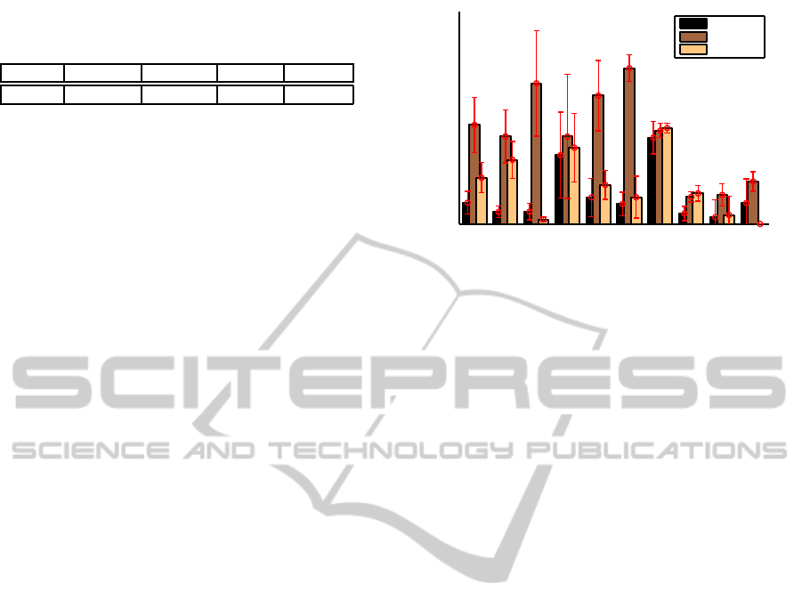
Table 2: Classification error rates (%) between the Multi-
view and traditional strategies for the USPS2 dataset.
Datasets Multi-view SemiBoost Modified S3VM-us
USPS2 0.42 20.87 28.03 27.27
labeled test set (T
e
), and unlabeled data set (U), with
a ratio of 20%: 20%: 60%. The training and test pro-
cedures were repeated ten times and the results were
averaged. The (Gaussian) radial basis function ker-
nel, i.e. Φ(x, x
′
) = exp(−(kx − x
′
k
2
2
)/2σ
2
), was used
for all algorithms. For simplicity, in the S3VM classi-
fier (which was implemented using the algorithm pro-
vided in (Chang, C. -C. and Lin, C. -J., 2011)), the
two constants, C
∗
and C, were set to 0.1 and 100, re-
spectively. The same scale parameter (σ), which was
found using cross-validation by training an inductive
SVM for the entire data set, was used for all meth-
ods. The proposed learning algorithm, in which a
S3VM was trained with L and U
s
selected using the
proposed criterion, was compared with three types
of traditional algorithms: SemiBoost, Modified, and
S3VM-us. In these S3VM algorithms, U
s
’s were se-
lected using the selection criteria provided in (Mal-
lapragada, P. K. et al., 2009), (Le, T. -B. and Kim, S.
-W., 2014), and (Li, Y. -F. and Zhou, Z. -H., 2011).
Also, the cardinality of U
s
’s was fixed as 10% of U.
4.3 Experimental Results obtained with
USPS2
In order to investigate the characteristics of the pro-
posed selection strategy, classification was performed
using the two-view USPS2 data, which has been syn-
thetically reconstructed from the original dataset.
Table 2 presents a numerical comparison of the
mean error rates (and standard deviations) (%) ob-
tained with the S3VM classifiers. Here, the results
in the second column (Multi-view) were obtained us-
ing the proposed learning algorithm (Algorithm 2).
The results of the third, fourth, and fifth columns were
obtained using the selection strategies of SemiBoost,
Modified, and S3VM-us, respectively.
From Table 2, the reader should observe that the
classification accuracy of S3VM could be signifi-
cantly improved when using the U
s
selected using
the multi-view based criterion. From this observa-
tion, the rationale that the multi-view based criterion
(Multi-view) developed in the present work, rather
than the distance and/or density based criteria (i.e.,
SemiBoost, Modified, and S3VM-us), has been em-
ployed as a selection strategy is clear.
0
0.1
0.2
0.3
0.4
0.5
0.6
0.7
0.8
0.9
Datasets
Wrong prediction rates
Aus
Cre
Eco
Gla
Hea
Pim
Qua
Seg
Veh
Vow
Multi−view
SemiBoost
Modified
Figure 2: Comparison of the wrong-prediction rates among
the three selection criteria for the experimental data. Here,
the datasets are represented with three letter acronym.
4.4 Wrong-prediction Rates: UCI
Datasets
Prior to presenting the classification accuracies, the
three criteria, i.e. newly proposed Multi-view, origi-
nal SemiBoost, and Modified, were compared. First,
the following question was investigated: does the
newly proposed selection criterion perform better
than the traditional criteria? To answer this question,
an experiment was conducted on labeling the unla-
beled data using the three selection criteria: a veri-
fication of the two predicted labels for each x
i
∈ U
using two criteria. As was done for the synthetic
data, the experiment was undertaken as follows: first,
a subset from U (i.e., U
s
) was selected using one
of the three criteria; second, the three labels of all
x
i
∈ U
s
were predicted using the three techniques in
(2), (3), and (4), i.e. sign(p
i
− q
i
), sign(ρ1(x
i
)),
and sign(ρ2(x
i
)) were compared with their true labels
(y
U
s
∈ {+1,−1}); the above two steps were repeated
ten times without increasing the cardinality of U
s
,
which means that, in Algorithm 2, for all j, ∆
( j)
= 0.
Fig. 2 presents a comparison of the ten values ob-
tained through performing the above experiment for
the UCI datasets. In the figure, the x-axis denotes UCI
datasets and the y-axis indicates the incorrect predic-
tion rates obtained using the three criteria.
From the figure, it can be observed that the pre-
diction capabilities of the three criteria differ from
each other; in general, the capability of the proposed
strategy, Multi-view, appears better than that of the
traditional strategies, SemiBoost and Modified. This
can be clearly demonstrated by comparing the wrong-
prediction rates in the figure. For almost all the
datasets, the lowest rate was observed with Multi-
view, rather than SemiBoost and Modified.
ICPRAM2015-InternationalConferenceonPatternRecognitionApplicationsandMethods
162

In addition to this observation, for Ecoli and
Vowel datasets, the prediction capability of Modi-
fied seems to be superior to that of Multi-view. This
means that the proposed strategy does not work well
with the two datasets. In order to discover the rea-
son for this poor performance, data complexities (Ho,
T. K. and Basu, M., 2002) were investigated as fol-
lows: first, two subsets of the UCI datasets, i.e. UCI1:
(Cre, Aus, Hea) and UCI2: (Eco, Vow) were con-
sidered; next, for the datasets of the two subsets, six
kinds of complexities, namely F3 (individual feature
efficiency), F4 (collective feature efficiency), N1 (the
fraction of points on the class boundary), N2 (ratio
of average intra/inter class nearest neighbor distance),
N3 (the leave-one-out error rate of the one-nearest
neighbor classifier, 1NN), and N4 (the nonlinearity
of 1NN) were measured. Details of the measurement
are omitted here in the interest of space, but observa-
tions obtained can be summarized as follows: for the
N measures, each value of UCI1 dataset is larger than
that of UCI2 dataset, whereas for the F measures, the
result is the opposite.
In review, as can be seen from Fig. 2, for a few
datasets, such as Ecoli and Vowel, the prediction ca-
pability of the proposed strategy seems to be infe-
rior to that of the traditional strategies, which means
that Multi-view does not work with certain kinds of
datasets. In order to figure out why this is, the data
complexities of the F and N measures were consid-
ered. From this measurement, it has been demon-
strated that the data sets, with which the new crite-
rion does not work, seem to be composed of similar
views, not different. From this observation, the rea-
son that the multi-view based criterion, rather than
the distance and/or density based criteria, has been
employed as a selection strategy, is clear again.
4.5 Experimental Results obtained with
UCI
In order to further investigatethe characteristics of the
proposed selection strategy and to determine which
types of datasets are more suitable for it, classifica-
tion was performed using the proposed and three tra-
ditional learning algorithms for the UCI datasets. In
particular, S3VM classifiers (Chang, C. -C. and Lin,
C. -J., 2011) were used. Here, the U
s
has been se-
lected using four different criteria: Mult-view, Semi-
Boost, Modified, and S3VM-us.
Table 3 presents a numerical comparison of the
mean error rates (and standard deviations) (%) ob-
tained with the S3VM classifiers. Here, the results in
the second column (Multi-view) were obtained using
the proposed learning algorithm (Algorithm 2). The
Table 3: Classification error rates (%) between the Multi-
view and traditional algorithms for the UCI datasets. Here,
the lowest error rate in each data set is underlined.
Datasets Multi-view SemiBoost Modified S3VM-us
Australian 27.23 39.05 36.06 32.41
Credit A 29.54 40.31 35.46 35.23
Ecoli 3.33 3.64 3.18 3.94
Glass 38.10 35.95 36.67 35.00
Heart 40.37 44.26 43.52 44.63
Pima 29.67 34.38 34.71 34.05
Quality 43.06 44.27 43.66 44.26
Segment 7.64 17.88 13.70 14.29
Vehicle 12.32 23.45 20.12 22.44
Vowel 5.05 12.76 4.38 5.71
results of the third, fourth, and fifth columns were
obtained using the selection strategies of the origi-
nal SemiBoost algorithm (Mallapragada, P. K. et al.,
2009), the modified SemiBoost algorithm (Le, T. -
B. and Kim, S. -W., 2014), and the S3VM-us algo-
rithm (Li, Y. -F. and Zhou, Z. -H., 2011) respectively.
For all algorithms, the cardinality of U
s
is 10% (i.e.,
α
( j)
= 10 for all j).
From Table 3, it should be observed that the clas-
sification accuracy of S3VM could generally be im-
proved when using theU
s
through the Multi-view cri-
terion. For example, consider the results for the Aus-
tralian dataset. For the dataset (d = 14), the lowest
error rate (27.23 %) was obtained using Multi-view.
However, as observed previously, the proposed crite-
rion did not work satisfactorily with certain kinds of
datasets, such as Ecoli, Glass, and Vowel.
Although it is hard to quantitatively compare the
four criteria, to render this comparative evaluation
more complete, we counted the numbers of the under-
lined error rates, obtained with the ten UCI datasets.
In summary, the numbers of the underlined error rates
for the four columns of Multi-view, SemiBoost, Mod-
ified, and S3VM-us are, respectively, 7, 0, 2, and 1.
From this, it can be observed that Multi-view, albeit
not always, generally works better than the others in
terms of the classification accuracy.
In addition to this simple comparison, in order
to demonstrate the significant differences in the error
rates among the selection criteria used in the experi-
ments, for the means (µ) and standard deviations (σ)
shown in Table 3, the Student’s statistical two-sample
test can be conducted. More specifically, using the t-
test package, the p-value can be obtained in order to
determine the significance of the difference between
the Multi-view and Modified criteria. Here, the p-
value represents the probability that the error rates of
the former are generally smaller than those of the lat-
ter. More details of this observation are omitted here,
but will be reported in the journal version.
OnSelectingUsefulUnlabeledDataUsingMulti-viewLearningTechniques
163

5 CONCLUSIONS
In an effort to improve the classification performance
of SSL based models, selection criteria with which
the models can be implemented efficiently were in-
vestigated in this paper. With regard to this concern,
various approaches have been proposed in the liter-
ature. Recently, for example, a selection strategy of
improving the accuracy of a SemiBoost classifier has
been proposed. However, the criterion has a weak-
ness, which is caused by the significant influence of
the unlabeled data when predicting the labels of the
selected examples. In order to avoid this weakness,
a selection strategy utilizing the multi-view learning
techniques was studied and compared with the origi-
nal strategy used for SemiBoost and its variants.
Experiments have been performed using synthetic
and real-life benchmark data, where the data was uni-
formly decomposed into two-views through a tradi-
tional feature selection method was applied for ex-
tracting the views. The experimental results obtained
demonstrated that the proposed mechanism can com-
pensate for the shortcomings of the traditional strate-
gies. In particular, the results demonstrated that when
the data is decomposed into multiple views efficiently,
i.e. the data has multiple different views as its real na-
ture, the strategy can achieve further improved results
in terms of prediction/classification accuracy.
Although it has been demonstrated that the ac-
curacy can be improved using the proposed strategy,
more tasks should be carried out. A significant task
is the decomposition of the multiple views from the
labeled and unlabeled data to measure correct confi-
dence labels of the unlabeled data. Furthermore, it is
not yet clear which types of datasets are more suitable
for using this multi-view based selection strategy for
SSL. Finally, the proposed method has limitations in
the details that support its technical reliability, and the
experiments performed were limited.
REFERENCES
Asuncion, A. and Newman, D. J. (2007). UCI Machine
Learning Repository. Irvine, CA. University of Cali-
fornia, School of Information and Computer Science.
Blum, A. and Mitchell, T. (1998). Combining labeled and
unlabeled data with co-training. In Proc. the 11th Ann.
Conf. Computational Learning Theory (COLT98),
pages 92–100, Madison, WI.
Chang, C. -C. and Lin, C. -J. (2011). LIBSVM : a library for
support vector machines. ACM Trans. on Intelligent
Systems and Technology, 2(3):1–27.
Chen, M., Weinberger, K. Q., and Chen, Q. (2011). Au-
tomatic feature decomposition for single view co-
training. In Proc. of the 28 th Int’l Conf. Ma-
chine Learning (ICML-11), pages 953–960, Bellevue,
Washington, USA.
Dagan, I. and Engelson, S. P. (1995). Committee-based
sampling for training probabilistic classifiers. In A.
Prieditis, S. J. Russell, editor, Proc. Int’l Conf. on Ma-
chine Learning, pages 150–157, Tahoe City, CA.
de Sa, V. (1994). Learning classification with unlabeled
data. In Advances in Neural Information Processing
Systems (NIPS), volume 6, pages 112–119.
Hastie, T., Tibshirani, R., and Friedman, J. (2001). The
Elements of Statistical Learning. Springer.
Ho, T. K. and Basu, M. (2002). Complexity measures of su-
pervised classification problems. IEEE Trans. Pattern
Anal. and Machine Intell., 24(3):289–300.
Kumar, A. and Daume III, H. (2011). A co-training ap-
proach for multi-view spectral clustering. In Getoor,
L. and Scheffer, T., editors, Proc. of the 28th Int’l
Conf. on Machine Learning (ICML-11), ICML ’11,
pages 393–400, New York, NY, USA. ACM.
Le, T. -B. and Kim, S. -W. (2014). On selecting help-
ful unlabeled data for improving semi-supervised sup-
port vector machines. In A. Fred, M. de Marsico,
and A. Tabbone, editor, Proc. the 3rd Int’l Conf. Pat-
tern Recognition Applications and Methods (ICPRAM
2014), pages 48–59, Angers, France.
Li, Y. -F. and Zhou, Z. -H. (2011). Improving semi-
supervised support vector machines through unlabeled
instances selection. In Proc. the 25th AAAI Conf. on
Artificial Intelligence (AAAI’11), pages 386–391, San
Francisco, CA.
Mallapragada, P. K., Jin, R., Jain, A. K., and Liu, Y.
(2009). SemiBoost: Boosting for semi-supervised
learning. IEEE Trans. Pattern Anal. and Machine In-
tell., 31(11):2000–2014.
Reitmaier, T. and Sick, B. (2013). Let us know your deci-
sion: Pool-based active training of a generative classi-
fier with the selection strategy 4DS. Information Sci-
ences, 230:106–131.
Yarowsky, D. (1995). Unsupervised word sense disam-
biguation rivaling supervised methods. In Proc. of
the 33rd annual meeting on Association for Compu-
tational Linguistics (ACL’95), pages 189–196, Cam-
bridge, MA.
Zhu, X. and Goldberg, A. B. (2009). Introduction to
Semi-Supervised Learning. Morgan & Claypool, San
Rafael, CA.
ICPRAM2015-InternationalConferenceonPatternRecognitionApplicationsandMethods
164