
Multi-objective Evolutionary Method for Dynamic Vehicle Routing
and Scheduling Problem with Customers' Satisfaction Level
Seyed Farid Ghannadpour and Mohsen Hooshfar
Department of Railway Engineering, MAPNA Co., Tehran, Iran
Keywords: Vehicle Routing Problem, Multi-Objective Optimization, Fuzzy Time Windows, Dynamic Request.
Abstract: This paper studies the multi-objective dynamic vehicle routing and scheduling problem by using an
evolutionary method. In this model, all data and information required to the routing process are not known
before planning and they revealed dynamically during the routing process and the execution of the routes.
Moreover, the model tries to characterize the customers’ satisfaction and the service level issues by
applying the concept of fuzzy time windows. The proposed model is considered as a multi-objective
problem where the overall travelling distance, fleet size and waiting time imposed on vehicles are
minimized and the customers’ satisfaction or the service level of the supplier to customers is maximized. To
solve this multi-objective model, an evolutionary algorithm is developed to obtain the Pareto solutions and
its performance is analyzed on various test problems in the literature. The computational experiments on
data sets represent the efficiency and effectiveness of the proposed approach.
1 INTRODUCTION
One of the most important combinatorial
optimization problems is the vehicle routing
problem with time windows (VRPTW) which is
seeking to service a number of customers with a
fleet of vehicles and pre-defined time windows. . In
this paper, the dynamic version of the VRP with
hard time windows and customers' satisfaction level
is considered. In this problem, customer orders for
service are called over time in a given planning
horizon and their location, size, and time window
become known only after they arrive. Obviously,
this type of problem is more challenging and
sophisticated than the conventional static VRPTW.
The literature of the VRPTW is rich in exact and
heuristic solution approaches. Applying meta-
heuristics (e.g., simulated annealing (SA), tabu
search (TS) and ant colony system) to solve the
VRPTW can be found in (Baños et al. 2013,
Cordeau and Maischberger 2012, Blaseiro et al.
2011). There are many papers used evolutionary
algorithms for the VRPTW (Ombuki et al. 2006,
Salhi and Petch 2007, Tan et al. 2006, Ghoseiri and
Ghannadpour 2010, and Ghannadpour et al. 2014).
In this regard, Tang et al. (2009) proposed and
solved a VRP with fuzzy time windows. Other very
good techniques and applications of the VRPTW
and its developments can be found in (Lei et al.
2011, Negata et al. 2010, Blaseiro et al. 2011,
Ghannadpour and Noori 2012). In the using of
dynamic approach of routing problems, many
authors developed different solution approaches
categorized in two major classes. One class of
methods, called a-priori optimization-based method,
is based on probabilistic information on future
events for service, customers demands, travel times,
etc. (Bent and Van Hentenryck 2004, Larsen et al.
2004). The other class of methods, called the real-
time optimization method, plans the routes solely
based on known information without looking into
the uncertain future (Chen and Xu 2006, Lorini et al.
2011,
and Haghani and Jung 2005).
Not many studies can be found in the literature
on multi-objective VRPTW. In this area Tan et al.
(2006) and Ombuki et al. (2006) and Ghoseiri and
Ghannadpour (2010) proposed a hybrid multi-
objective evolutionary algorithm with the concept of
Pareto’s optimality. Najera and Bullinaria (2011)
proposed and analyzed a novel MOEA, which
incorporates methods for measuring the similarity of
solutions. The remainder of this paper is organized
as follows. Section 2 defines the model. The solution
technique is discussed in Section 3. Section 4
91
Farid Ghannadpour S. and Hooshfar M..
Multi-objective Evolutionary Method for Dynamic Vehicle Routing and Scheduling Problem with Customers’ Satisfaction Level.
DOI: 10.5220/0005172600910098
In Proceedings of the International Conference on Operations Research and Enterprise Systems (ICORES-2015), pages 91-98
ISBN: 978-989-758-075-8
Copyright
c
2015 SCITEPRESS (Science and Technology Publications, Lda.)

describes the computational experiments. Section 5
provides the concluding remarks.
2 PROPOSED DYNAMIC MODEL
In dynamic VRPTW all data and information
required to the routing process are not known before
planning and they revealed dynamically during the
routing process and the execution of the routes. So,
the planner encounters with the information of the
limited number of customers at the beginning of the
planning. During the routing process, new requests
can arrive in the system. Thus, the dynamic VRPTW
is strongly related to the static VRPTW. The
DVRPTW can be consequently modelled as a
sequence of the static VRPTW-like instances. In
particular, each static VRPTW will contain all the
customers known at that time, but not yet served.
The most important data for the re-optimization
stage are relevant to information regarding real time
requests and dispatched vehicles. The information
required for new customers is identified when they
call in for services to a dispatch center. However, the
vehicular information is determined by constant
communication between vehicles and the depot. In
addition, when the dispatching center knows the last
state of a vehicle at any time, it will have to re-
optimize the routing plan with new information. In
practice, transportation often
characterizes the service
level issues and
involves routing vehicles according to
customer-specific time windows, which are highly
relevant to the customers’ satisfaction level. In these
many realistic applications, the concept of classical
time windows does not model the preference of
customers very well. Even though customers provide
a fixed time window for service, they really hope to
be served at a desired time if possible. This
preference information of customers can be
represented as a convex fuzzy number with respect
to the satisfaction for service time. This concept
changes the classical hard time window [e
i
, l
i
] to the
triple [e
i
, u
i
, l
i
]. The membership function of
customer i or
()
ii
t
, which represents the grade of
satisfaction when the start of service time is t
i
defined by triangular membership function. The start
of service time is
,
where f
i
is the
service time of customer i and T
i-1,i
is the travel time
between customer i-1 and customer i. when
,
the start of service time is
considered
and the vehicles undergo a waiting
time.
Moreover, the proposed model is considered as a
multi-objective problem where the overall travelling
distance, fleet size and waiting time imposed on
vehicles are minimized and the
customers’
satisfaction or the service level of the supplier to
customers is maximized. These objectives are
(
Min
∑∑ ∑
.
∈∈,∈
and
Min
∑∑
∈∈,
, where N and K are
the set of customers and vehicles, respectively. For
simplicity, the depot is denoted as customer 0. The
travel distance between customers i and j is denoted
as
. Moreover, the decision variable
is equal
to 1 if vehicle k drives from customer i to customer
j, and 0 otherwise. Moreover, the model tries to
serve all the customers such that the summation of
their satisfaction rates is maximized as
Max
∑
∈
. When the arrival time of vehicles is
before e
i
, they undergo a waiting time that is
desirable and affects more vehicle and labour costs,
The summation of this waiting time, should be
minimized according to
Min
∑
∈
), where
the waiting time imposed on each vehicle for
customer i is calculated by
w
t
t
f
T
,
. Eventually, the multi-objective problem
(MOP) studied in this paper is stated by:
(1)
F
x
f
,
f
,
f
,
f
s.t.x
∈ D
Where x
is the decision variable vector, D is
space, and F
x
is the objective vector. The solution
to a MOP is the set of non-dominated solutions,
called the Pareto set (PS). Eventually, this paper
uses a posteriori approach, in which a set of
potentially non-dominated solutions is first
generated, and then the decision-maker chooses
among those solutions
3 SOLUTION PROCEDURE
A solution procedure consisting of three basic
modules is developed to solve the proposed model:
management module, strategy module and
optimization module.
3.1 Management Module
The management module tries to check the state of
the system including information of vehicles and
customers each time. The customers’ information
includes geographical location (
,
), the on-site
service time, the demand (
and time window of
each customer. Initially, at time 0, the pool of
the customers’ information may consist of all
ICORES2015-InternationalConferenceonOperationsResearchandEnterpriseSystems
92
determined request customers who are remained
from the previous working day and they should be
served today. As time elapses (0), this pool of
request is enlarged if a new customer for service is
received and reduced whenever the service of a
request or customer is ended. Thus, the management
module tries to control the customers' information as
,
,
,
,
,
,
,
, where
is the call
time of customer (i) with the central dispatching
center and it is considered 0 for the determined
customers. It should be noted that the planning
horizon is considered as
0,. Initially all vehicles
are located at depot and all required information is
available. As time elapses (
0), the management
module should control the state of dispatched
vehicles and update their information continually for
subsequent planning. The information, which should
be checked by a dispatcher, includes the
geographical locations, the residual capacity, the
state of vehicle (i.e., driving, servicing, and waiting),
and the like.
3.2 Strategy Module
The strategy module tries to organize the
information reported by management module and
construct an efficient structure for solving in the
subsequent phase (optimization module). Therefore,
the K discrete time periods are considered in each
working day as
,
,…,
where,
0
⋯
. Moreover, each time slice represents a
partial static VRP with fuzzy time windows and is
defined as
1∆ where, 1,…, and ∆
(∆ 0) is the time interval between two consecutive
steps. It should be noted that ∆ depends on the
degree of system dynamism. The designed
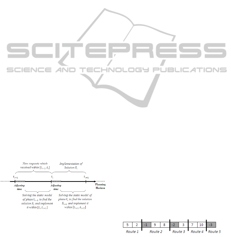
procedure is illustrated in Figure 1.
Figure 1: Dynamic structure for the proposed model.
According to this figure, in each time step t
, a
certain amount of times (δ) as adjusting time should
be spent to construct the static model. This model is
solved within
,
to find the solution
,
which should be implemented in the next time slice
and within
,
. Moreover, in time step
,
solution
found in the previous time step (
,
) is implemented within
,
. The required
information for constructing the partial static model
in time step
is relevant to information of
customers and vehicles reported by management
module. The set of vehicles information that should
be considered in time slice
, is as
∪
, where,
is the set of vehicles en routes until
with the
information of their status, residual capacity and
geographical location. The dispatching time of new
vehicles solution
is
and their horizon of
planning is set as
,. Moreover, the set of
customers’ information, which is necessary for
finding the solution
within
,
, is as
\
∪
, where
is the set of
customers considered in previous time slice
and
is the set of customers which are served within
,
by implementing of solution
. Moreover,
is the set of new customers, which called in for
service within
,
.
3.3 Optimization Module
The optimization module solves each static model of
time slice
within
,
and passes the new
solution vector on to the management and strategy
modules for updating and implementing. Naturally,
changes can only be made to the unvisited parts of
the routes. As mentioned earlier, the modified GA,
which was developed in our recent research
(Ghoseiri and Ghannadpour 2010) is used here.
3.3.1 Representation
A solution of the model in time slice
, which no
vehicles have been commissioned yet, is represented
by an integer string of length
, where
is the
number of determined requests remained from the
previous working day. On the subsequence time
slices
(1), some customers are visited during
the previous slices and some others are waiting for
services. The solution representation of these time
slices is a variable length chromosome
representation as depicted in Figure 2.
Figure 2: Chromosome representation of step t
(i1).
Multi-objectiveEvolutionaryMethodforDynamicVehicleRoutingandSchedulingProblemwithCustomers'Satisfaction
Level
93

Two types of nodes are used in this representation,
namely positive and negative nodes. The positive
nodes represent the unvisited and new customers
that have been added to this day’s schedule
during
,
. The negative nodes represent the
group of clustered customers that have already been
visited by the dispatched vehicles during the
previous time slices. So these negative nodes are the
indices of dispatched vehicles as a place holder and
include the information of their partial routes and
previously visited customers. When this
chromosome is decoded, new customers can be
added to these pre-existing routes if they still satisfy
the feasibility conditions.
3.3.2 Pareto Ranking Procedure
The Pareto ranking procedure (Ghoseiri and
Ghannadpour 2010) which tries to rank the solutions
to find the non-dominated solutions is used for
evaluation of each chromosome. In this approach,
chromosomes assigned rank 1 are non-dominated,
and inductively, those of rank i +1 are dominated by
all chromosomes of ranks 1 through i.
3.3.3 Recombination
The best cost -best route crossover (BCBRC) and
sequenced based mutation (SBM) are used as
recombination operators (Ghoseiri and Ghannadpour
2010). This paper uses the modified best cost-best
rout crossover (BCBRC), which selects a best route
from each parent and then for a given parent, the
customers in the chosen route from the opposite
parent are removed. The final step is to locate the
best possible locations for the removed customers in
the corresponding children.
3.3.4 Local Search
This paper uses a -interchange mechanism as local
search method that moves customers between routes
to generate neighborhood solution for the proposed.
In one version of the algorithm called GB (global
best), the whole neighborhood is explored and the
best move with lower rank is selected. In another
version, FB (first best), the first admissible
improving move is selected if exists; otherwise the
best admissible move is implemented.
3.3.5 Satisfaction Improvement Operator
The satisfaction improvement operator (SIO) is used
to improve the satisfaction rate of each customer
without increasing the waiting time and by pushing
the waiting time of vehicles on each customer along
the routes. This push will increase the total degree of
satisfaction along the route without violating the
feasibility conditions. In general, the SIO operator is
applied on the chromosomes with the following
characteristics: 1- the solutions has at least one
vehicle with non-zero waiting time, 2- If a vehicle
incurs more than one
along a route, the route
should be devided into some sections (each section
is named “path”) according to the number of
vehicles waiting time and 3- All the derivative terms
of the customers or the slope of satisfaction function
at time
for customers is larger than zero. then a
possible forward push will cause the increase of total
grade of satisfaction. The feasible forward push in
each step is as
,, where Δ
,if
and Δ
,if
.
After applying this push, the part of the path from
the Customer
*
to end is considered again and the
above characteristics are checked. The Customer
*
is
the customer that the previous minimum push has
been found on it. This procedure is repeated until
the new feasible forward push cannot be found.
4 COMPUTATIONAL ANALYSIS
At the beginning, the proposed model is considered
in static conditions with two objectives that
minimize the total distance travelled and the total
number of vehicles, which are the most common
objectives used by other researchers alternatively.
After that two another defined objective functions,
are added and the developed model is considered in
dynamic conditions. The experimental results use
the standard Solomon’s VRPTW benchmark
problem instances that are available in (Solomon
1987). The proposed algorithm is coded and run on a
PC with Core 2 Duo CPU (3.00 GHz) and 2.9 GB of
RAM. Moreover, the model is implemented under
parameters of Population size = 100, Generation
number = 1000, Crossover rate = 0.80, Mutation rate
= 0.40, Improve the solution by 2-interchange (GB)
and 1-interchange (FB) operators, Selection rate of
improvement operators = 0.5 and Repetition for
experiments = 5. Table 1 presents a summary of
results. The average number of vehicles (upper
figure) and the average travel distance (lower figure)
of the best known results (Blaseiro et al. 2011) and
Ghoseiri and Ghannadpour 2010) and the proposed
method are presented in this Table. Additionally, the
last row presents, the total number of vehicles and
total travel distance for all 56 instances. Moreover,
two series of results are presented in this table for
ICORES2015-InternationalConferenceonOperationsResearchandEnterpriseSystems
94

proposed method, one corresponding to the solutions
with smallest number of vehicles (min V) among the
non-dominated solutions and the other regarding
solutions with the shortest travel distance (min D).
According to this table, the proposed method
obtained the very good results for sets C1 and C2.
On the other hand, for the remaining categories,
solutions from the proposed method are between
1.79% and 5.27% larger in distance cost than the
best results, and consider 3.25% and 5.74% more
vehicles (for category R1 and RC1).
Table 1: Average results of proposed method and the best
known solutions.
Pro.
Best
known
Proposed
(Min V)
Proposed
(Min D)
%
diff. V
% diff.
D
C1
10.00
828.38
10.00
828.38
10.00
828.38
0.00 0.00
C2
3.00
589.77
3.00
591.49
3.00
591.49
0.00 0.29
R1
12.50
1195.15
12.92
1228.60
13.50
1217.03
3.25 1.79
R2
3.36
905.60
3.27
1066.15
4.00
956.08
-
2.75
5.27
RC
1
12.13
1361.86
12.87
1390.06
13.25
1384.30
5.74 1.62
RC
2
4.00
1052.84
3.75
1114.19
4.00
1109.20
-
6.66
5.08
total
430
55794.58
438
58692.32
458
57256.65
1.82 2.55
But for categories R2 and RC2 the better number
of vehicles is obtained in average of 2.75% and
6.66% than the best known respectively. Moreover,
the difference between the results of proposed
method and best known solutions for all 56 instances
is only 1.82% and 2.55% for the number of vehicles
and travelled distance respectively. The average
computational time for classes C1, R1 and RC1
varies between 2 and 3 hours with 1000 generations
and is between 5 and 7 hours for classes C2, R2 and
RC2. The second classes require a larger CPU time
due to the longer time windows, which allow a more
flexible arrangement in the routing construction
process. Moreover, an operator deletion- retrieval
strategy is executed to probe the efficiency of the
inner working of the proposed method. According to
this strategy, genetic operators are eliminated one at
a time and each time, algorithm is put into run and
convergence behaviour is studied and compared
with the operator retrieved. The results of instance
C203 with respect to the shortest travel distance is
represented as Figure 3. According to this figure, all
the inner components of the genetic algorithm work
properly and indicate good behaviour of
convergence toward the best solutions. Among these
operators, the Hill-climbing operator works highly
efficient to convergence toward the best solution.
Now the fuzzy time windows are considered
instead of classical time windows and the proposed
model should be implemented with four defined
objective functions in a multi-objective manner and
in static conditions. It should be noted that in some
experiments there are more than 50 or 60 non-
dominated solutions.
Figure 3: Inner working of proposed method for C203.
In general, the relationship between defined
objectives in a routing problem is unknown until the
problem is solved in a proper multi-objective
manner. These objectives may be positively
correlated with each other or they may be conflicting
to each other. Based on the results, all instances in
the category C have the positively correlating
objectives when the first two objectives are
considered. In general, it can be expressed that the
multi-objective manner is not required for the C
category due to have the correlating objectives. But
the conflicting behaviours are more in R and RC
categories and most of these instances have the
conflicting objectives in a population distribution of
them. For instance the behaviour of instance R103 is
shown in (Figure 4 a, b, c), which is the population
distribution with respect to the distance cost, total
satisfaction rate and waiting cost.
According to Figure 4-a, the customers'
satisfaction rate is improved as the total travelling
distance cost is deteriorated. Figure 4-b illustrates
the population distribution of this problem with
respect to the distance and waiting cost. Moreover,
the relationship of the waiting cost and customers'
satisfaction rate for problem R103 is illustrated in
Fig. 4-c. In spite of the designed algorithm and
operators (SIO) trying to improve the satisfaction
rate of customers by using the current waiting time,
Multi-objectiveEvolutionaryMethodforDynamicVehicleRoutingandSchedulingProblemwithCustomers'Satisfaction
Level
95
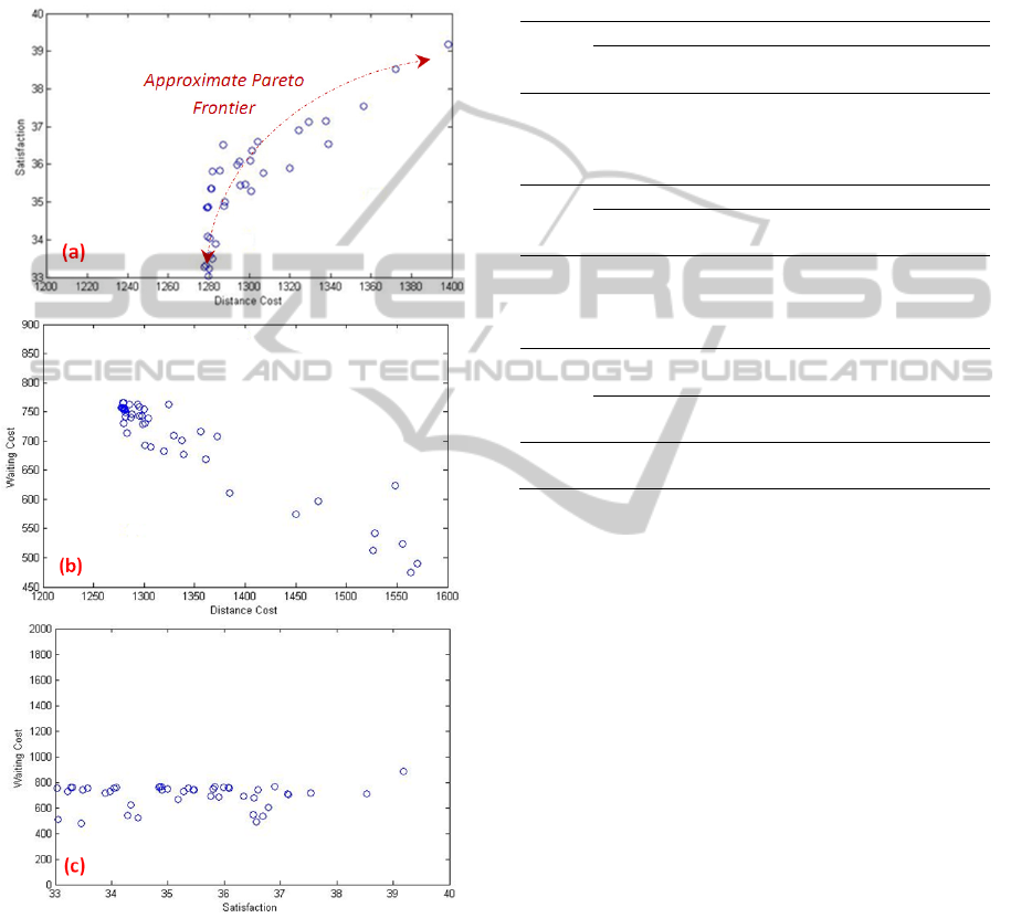
these two objectives are independent of each other.
This is due to the nature of the first categories of the
Solomon's instances that have much lower waiting
time than the second classes in general. For
example, in problem R204 the summation of the
customers' satisfaction rate is increased by more
waiting cost.
Figure 4: Comparison of non-dominated solutions of
problem R103.
For more appropriate comparison, the
performance of proposed evolutionary method is
also compared with standard NSGA-II. The
principals and the concept of this method could be
found in Deb (2002). Table 2 presents the average
results of the non-dominated solutions found by
these methods. It should be noted that the
comparisons are done on whole data sets of Class R
and some of which are reported in this Table for the
sake of brevity. Moreover, the deviation between the
average results of each method on whole data sets of
Class R is listed in the last rows.
Table 2: Comparison between the proposed evolutionary
method and NSGA-II.
Pro.
Proposed Method – Average Results
Distance
Cost
Vehicle #
Customers'
satisfaction
Waiting
Cost
R103
R108
R203
R204
Pro.
NSGA-II – Average Results
Distance
Cost
Vehicle #
Customers'
satisfaction
Waiting
Cost
R103
R108
R203
R204
Data
Sets
Deviation (%) of proposed method from
NSGA-II
Distance
Cost
Vehicle #
Customers'
satisfaction
Waiting
Cost
Class
R
- 4.8 -1.1 -6.1 -15.9
Based on our analysis the computational efforts
of proposed method are near to NSGA-II. Moreover
the average results found by the proposed method
represents the competitive improvements according
to Table 2. The deviations are also calculated based
on the findings and the negative values represent the
improvement occurred by the proposed method in
comparison with NSGA-II. According to this table
the average difference between the proposed method
and NSGA-II illustrates the improvement of 4.8% in
the first objective, 1.1% in the second, 6.1% in the
third, and 15.9% in the fourth objective. The
significant improvement on the last two functions is
due to use of Satisfaction Improvement Operator
(SIO) that tries to increase satisfactions without
increasing the waiting time.
Now, the proposed model should be checked in
a dynamic structure. As observed before, at the end
of each stage
, a set of non-dominated solutions
are generated. By the displaced ideal method
considering the LP metric, one solution is chosen
from all non-dominated solutions (
) to
implement in the next time slice and
within
,
. Moreover, the call-in time for
each customer is uniformly distributed in the
following interval:
ICORES2015-InternationalConferenceonOperationsResearchandEnterpriseSystems
96
(2)
0.5∗min
,
2∆
,
min
,
2∆)]
Where,
is the travelling time from the depot
to customer i, and ∆ is the time between two
consecutive decision stages. It should be noted that
all the requests or customers with non-positive call-
in time are considered as determined requests.
The results are reported in Table 3. According
to this Table, each instance is solved in two different
cases. In the first case, the planning horizon is
divided into three decision stages (∆ 3), and in the
other case it is divided into five decision stages
(∆ 5). Obviously, the time between two
consecutive decision stages (∆) of the first case is
less than that in the second case.
Table 3: Testing results of the Solomon's instances for the
multi-objective dynamic VRPFTW.
Pro.
∆ 3
Distance
Cost
Vehicle #
Customers'
satisfaction
Waiting
Cost
R103 1833.12 20 36 608.12
R108 1231.8 13 50.7 355.1
R203 1820 9 46.6 2011
R204 1001.5 6 47.1 1520.01
RC101 2219.1 21 36.1 788.5
RC105 2010.5 20 42.5 720.5
Pro.
∆ 5
Distance
Cost
Vehicle #
Customers'
satisfaction
Waiting
Cost
R103 1854.32 20 36.5 622.71
R108 1596.4 15 52 374.2
R203 1801.2 9 47 1987
R204 986.82 6 48 1486.8
RC101 2275.4 22 36.3 743.32
RC105 2096.1 20 43 714.2
According to this Table, the quality of the
solutions in the dynamic environment is generally
lower than solutions in a static environment.
Moreover, this quality is strongly dependent on the
method by which customers entering and calling to
the decision system. Moreover, according to this
table, the quality of the solutions is also dependent
on the amount of time between two consecutive
decision stages (∆) too. This quality is improved
whenever this stage is longer, because the algorithm
has more time to solve the partial static model.
Therefore, in the systems with a high degree of
dynamism, the reaction time for services to real-time
requests is very short, and thus therefore the cost of
finding a new solution is increased. In this situation,
when ∆ is very small, the simple heuristics (e.g.,
insertion methods) can be used.
5 CASE STUDY
The proposed model is under implementation for
locomotives routing and assignment for railway
transportation division of MAPNA Group. In this
paper the results obtained on this real application for
the routes of Tehran – Mashhad are reported briefly.
This route is one of the most critical and important
routes and the two main and the largest cities of
country are connected by this railway route. In this
model the trains are considered as customers and
they are made up at different stations of network and
they need to receive locomotive based on the time
table of train scheduling. Moreover, the locomotives
are located at some central depots and they depart
toward the trains to move them from their origins to
their destinations based on the train scheduling
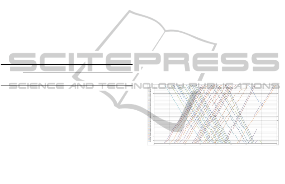
tables. The train scheduling plan of Tehran –
Mashhad railway routes is illustrated in Figure 5. By
this plan all the fuzzy time windows for trains could
be identified.
Figure 5: train scheduling plan of Tehran - Mashhad.
In this case, the trains with low priorities are
considered to be having the classical time windows.
Moreover, the trains with highly priority have the
fuzzy time windows and the desired time is nearest
to the earliest dispatching time of each train. The
dynamic trains which they made up out if pre-
defined plan use the narrow fuzzy time windows,
which indicate the willingness of these requests in
order to receive their services as soon as possible. At
present, 185 trains with different priorities are in
Tehran – Mashhad railway routes and more than 126
locomotives are required to serve them. The
proposed approach is applied on this route when the
two dynamic trains with different priorities are made
up every day. Moreover the model is implemented
for a week by the proposed dynamic structure and
detailed schedules of required locomotives are
planned. Based on the results, only 78 locomotives
are required to serve the whole trains of this route
and the total operational costs related to locomotives
is significantly decreased. The waiting time of
Multi-objectiveEvolutionaryMethodforDynamicVehicleRoutingandSchedulingProblemwithCustomers'Satisfaction
Level
97

locomotives is totally decreased by 35% and it has a
significant impact on reducing costs as well.
Moreover, the detailed schedule of each locomotive
including the departure time, trains in its
commitments, planned routes, waiting times and etc
is corresponding to the routes found by the proposed
VRPTW and they are identified for this route.
6 CONCLUSIONS
In this paper, a new multi-objective dynamic vehicle
routing and scheduling problem has been presented
and solved. To solve this multi-objective model, an
evolutionary algorithm has been and its performance
has been analyzed on various test problems. The
results show the efficiency and effectively of
proposed method. Finally, the real case study has
been considered by the proposed model as well and
it has been analyzed.
ACKNOWLEDGEMENTS
The authors would like to thank MAPNA Group for
its supports and financing this paper.
REFERENCES
Baños, R., Ortega, J., Gil, C., Fernández, A., Toro, F.,
2013. A Simulated Annealing-based parallel multi-
objective approach to vehicle routing problems with
time windows. Expert Systems with Applications 40:
376-383.
Bent, R., W., and Van Hentenryck, P., 2004. Scenario-
based planning for partially dynamic vehicle routing
with stochastic customers. Operations Research 52:
977–987.
Blaseiro, S.R., Loiseau, I., and Ramonet, J., 2011. An ant
colony algorithm hybridized with insertion heuristics
for the time dependent vehicle routing problem with
time windows. Computers and Operations Research
38(6): 954–966.
Blaseiro, S.R., Loiseau, I., Ramonet, J., 2011. An ant
colony algorithm hybridized with insertion heuristics
for the time dependent vehicle routing problem with
time windows. Computers and Operations Research
38: 954–966.
Chen, Z.L., and Xu, H., 2006. Dynamic column generation
for dynamic vehicle routing with time windows.
Transportation Science 40: 74-88.
Cordeau, J.F., Maischberger, M., 2012. A parallel iterated
tabu search heuristic for vehicle routing problems.
Computers and Operations Research 39: 2033-2050.
Deb, K., 2002. A fast and elitist multiobjective genetic
algorithm: NSGA-II. IEEE Transaction on
Evolutionary Computation 6: 182-197.
Garcia-Najera, A., and Bullinaria, J.A., 2011. An
improved multi-objective evolutionary algorithm for
the vehicle routing problem with time windows.
Computers and Operations Research 38: 287–300.
Ghannadpour, S.F., and Noori, S., 2012. high-level relay
hybrid metaheuristic method for multi-depot vehicle
routing problem with time windows. Journal of
Mathematical Modelling and Algorithms 11: 159-179.
Ghannadpour, S.F., Noori, S., Tavakkoli Moghaddam, R.,
Ghoseiri, K., 2014. A multi-objective dynamic vehicle
routing problem with fuzzy time windows: Model,
solution and application. Applied Soft Computing 14:
504-527.
Ghoseiri, K., and Ghannadpour, S.F., 2010. Multi-
objective vehicle routing problem with time windows
using goal programming and genetic algorithm.
Applied Soft Computing 4: 1096-1107.
Haghani, A., Jung, S., 2005. A dynamic vehicle routing
problem with time-dependent travel times. Computers
and Operations Research 32: 2959-2986.
Larsen, A., Madsen, O. B. G., Solomon, M.M., 2004. The
a-priori dynamic traveling salesman problem with time
windows. Transportation Science 38: 459–572.
Lei, H., Laporte, G., Guo, B., 2011. The capacitated
vehicle routing problem with stochastic demands and
time windows. Computers and Operation Research
38: 1775-1783.
Lorini, S., Potvin, J-Y., Zufferey, N., 2011. Online vehicle
routing and scheduling with dynamic travel times.
Computers and Operations Research 38: 1086–1090.
Negata, Y., Braysy, O., Dullaret, W., 2010. A penalty-
based edge assembly memetic algorithm for the
vehicle routing problem with time windows.
Computers and Operations Research 37: 724 – 737.
Ombuki, B., Ross, B., Hanshar, F., 2006. Multi-Objective
Genetic Algorithm for Vehicle Routing Problem with
Time Windows. Applied Intelligence 24: 17-30.
Salhi, S., Petch, R.J., 2007. A GA based heuristic for the
vehicle routing problem with multiple trips. Journal of
Mathematical Modelling and Algorithms 6: 591-613.
Solomon, M.M., 1987. Algorithms for the vehicle routing
and scheduling problems with time window
constraints. Operations Research 35: 254–265.
Tan, K.C., Chew, Y.H., Lee, L.H., 2006. A hybrid
multiobjective evolutionary algorithm for solving
vehicle routing problem with time windows.
Computational Optimization and Applications 34:
115-151.
Tanga, J., Pana, Zh., Fung, R.Y.K., Laus, H., 2009.
vehicle routing problem with fuzzy time windows.
Fuzzy Sets and Systems 160: 683–695.
ICORES2015-InternationalConferenceonOperationsResearchandEnterpriseSystems
98
