BLSTM-CTC Combination Strategies for Off-line Handwriting

Recognition

L. Mioulet

1,2

, G. Bideault

, C. Chatelain

, T. Paquet

and S. Brunessaux

Laboratoire LITIS - EA 4108, Universite de Rouen, 76800 Saint-

Etienne-du-Rouvray, France

Airbus DS, Parc d’affaires des Portes, 27106 Val de Reuil, France

Laboratoire LITIS - EA 4108, INSA Rouen, 76800 Saint-

Etienne-du-Rouvray, France

Keywords:

Feature Combination, Recurrent Neural Network, Neural Network, Handwriting Recognition.

Abstract:

In this paper we present several combination strategies using multiple BLSTM-CTC systems. Given several

feature sets our aim is to determine which strategies are the most relevant to improve on an isolated word

recognition task (the WR2 task of the ICDAR 2009 competition), using a BLSTM-CTC architecture. We

explore different combination levels: early integration (feature combination), mid level combination and late

fusion (output combinations). Our results show that several combinations outperform single feature BLSTM-

CTCs.

1 INTRODUCTION

Automatic off-line handwriting recognition is the

transcription into an electronic format of an image

containing a graphical representation of a word. The

recognition of ofﬂine handwriting is difﬁcult due to

the variability between writers for a same word, pres-

ence of overlapping letters, and complex long term

context dependencies. However, handwriting systems

have been successfully applied to different tasks, such

as bank cheque recognition (Knerr et al., 1997) and

postal address recognition (El-Yacoubi et al., 1995).

Indeed bank cheques and addresses follow a strict for-

mat and have a very limited vocabulary: the prior

knowledge on these task is extensively used to boost

the recognition performances. However, the recogni-

tion of unconstrained handwriting that can occur in

various documents, such as letters, books, notes, is a

very complex task. Exploring recognition in context

free systems is now a main interest of researchers.

Handwriting systems are generally divided in four

steps: preprocessing, feature extraction, recognition

and post-processing. In this paper we focus on the

recognition stage, for which the Hidden Markov Mod-

els (Rabiner, 1989) (HMM) have been massively used

(Kundu et al., 1988; El-Yacoubi et al., 1999; Bunke

et al., 2004). HMMs are states machines that com-

bine two stochastic processes: a stochastic event that

cannot be observed directly (the hidden states) is ob-

served via a second stochastic process (the observa-

tions).

These models have several advantages. First they

provide a way of breaking out of Sayre’s paradox

(Vinciarelli, 2002). Indeed recognizing a letter in a

word image requires its prior detection. But the re-

verse is also true, thus leading to an ill posed problem

known as Sayre’s paradox in the literature. Methods

using HMMs break up word images in atomic parts,

either as graphemes or frames extracted using a slid-

ing window. This will cause a difference between

the input sequence length and the output sequence

length. However, HMMs are able to cope with this

difference in length, they can label unsegmented se-

quences. They do so by recognizing every window as

a character or part of a character and modeling char-

acter length. A second advantage of HMMs is their

robustness to noise since they are statistical models.

Furthermore, the algorithms used for HMMs decod-

ing integrate language modeling, lexicon check or N-

gram models, which makes them very powerful tools

for handwriting recognition.

However, they also have some shortcomings.

Firstly, they are generative systems, which means that

when compared to other classiﬁers, they have a lesser

ability to discriminate between data since they pro-

vide a likelihood measure to decide . Secondly, within

the HMMs framework the current hidden state only

depends on the current observation and the previous

173

Mioulet L., Bideault G., Chatelain C., Paquet T. and Brunessaux S..

BLSTM-CTC Combination Strategies for Off-line Handwriting Recognition.

DOI: 10.5220/0005178601730180

In Proceedings of the International Conference on Pattern Recognition Applications and Methods (ICPRAM-2015), pages 173-180

ISBN: 978-989-758-076-5

 2015 SCITEPRESS (Science and Technology Publications, Lda.)

state (markovian condition) which prohibits the mod-

eling of long term dependencies.

Recently a new system based on recurrent neural

networks (Graves et al., 2008) has overcome these

shortcomings. The Bi-directional Long Short Term

Memory neural network (Hochreiter and Schmidhu-

ber, 1997; Gers and Schraudolph, 2002) (BLSTM)

consists in combining two recurrent neural networks

with special neural network units. The output of

these networks are then processed by a special Soft-

max layer, the Connectionist Temporal Classiﬁcation

(Graves and Gomez, 2006) (CTC), that enables the

labelling of unsegmented data. The composed sys-

tem, referred as the BLSTM-CTC, has shown very

impressive results on challenging databases (Graves,

2008; Graves et al., 2009; Grosicki and Abed, 2009;

Menasri et al., 2012).

In this paper, we present three baseline systems

using the same architecture, built around the BLSTM-

CTC network. These systems only differ by the

features that are extracted using a sliding window

method. These baseline systems enable a direct com-

parison between the three sets of features, which en-

ables us to prefer one set of features over the other.

However, it is well known that combining systems

or features may improve the overall results (Menasri

et al., 2012; Gehler and Nowozin, 2009).

In this paper we explore different ways of com-

bining an ensemble of F BLSTM-CTC. We explore

different levels of information combination, from a

low level combination (feature space combination), to

mid-level combinations (internal system representa-

tion combinations), and high level combinations (de-

coding combinations). The experiments are carried

out on the handwriting word recognition task WR2

of the ICDAR 2009 competition (Grosicki and Abed,

2009). We ﬁrst present the baseline system used for

handwriting recognition. We then detail the differ-

ent level of combinations available throughout the

BLSTM architecture, ﬁnally we present the results

and analyse them.

2 THE BASELINE PROCESSING

SYSTEM

In this section we present the baseline system we use

to recognize handwritten word images. We ﬁrst give

an overview of our system, we then describe each step

with further detail.

2.1 Overview

Our system is dedicated to recognizing images of iso-

lated handwritten words. In order to do so we imple-

mented a very common processing workﬂow that is

represented in Fig. 1.

First the image is preprocessed in order to remove

noise and normalize character appearance between

different writing styles. Given that our main interest

is the combination of systems we did not focus on the

preprocessing, hence we used well known algorithms

that have been widely used in the literature. After

cleaning the image we use a sliding window to ex-

tract the features: a window of length P is used to ex-

tract a subframe from the image, this subframe is then

analyzed and transformed by mathematical processes

into a M dimensional vector representation. For in-

stance a 2D image of length N is transformed into a

sequence of N feature vectors of dimension M.

This sequence is then processed by a BLSTM-

CTC network, in order to transform this M dimen-

sional signal into a sequence of labels (characters).

This output is ﬁnally processed by a HMM in order

to apply a directed decoding. It has to be stressed

that it is possible to add a lexicon to the BLSTM-CTC

(Graves et al., 2009) decoding stage. However, we did

not opt for this solution since the HMMs enable us to

be more modular, e.g. offering the possibility to inte-

grate language models with various decoding strate-

gies available on standard decoding platforms such as

HTK (Young et al., 2006), Julius (Lee et al., 2001) or

Kaldi (Povey et al., 2011), without deteriorating the

performances.

We now go into further details for each part.

2.2 Preprocessing

The preprocessing of images consists in a very simple

three step image correction. First a binarization by

thresholding is applied. Secondly a deslanting pro-

cess (Vinciarelli and Luettin, 2001) is applied. The

image is rotated between [−Θ;Θ] and for each an-

gle θ the histogram of vertical continuous traits H

measured. The deslanting angle is determined by the

with the maximum number of continuous traits.

Thirdly a height normalization technique is applied to

center the baseline and normalize the heights of the

ascenders and descenders.

2.3 Feature Computation

Among numerous feature representations, we se-

lected three efﬁciency proven features: the pixels, the

features presented in (Graves et al., 2009), and the

ICPRAM2015-InternationalConferenceonPatternRecognitionApplicationsandMethods

174

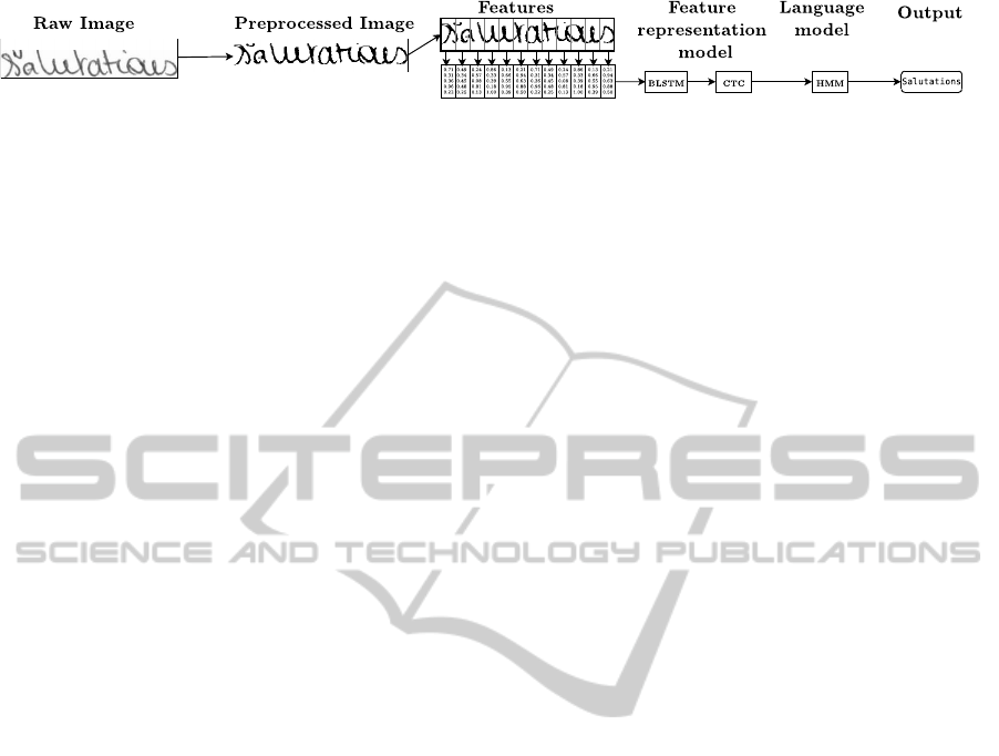
Figure 1: The baseline system.

Histogram of Oriented Gradients (Dalal and Triggs,

2005; Ait-Mohand et al., 2014). In the remaining of

this paper, these feature sets are respectively referred

as Pixels, SPF and HOG. They are all extracted us-

ing a sliding window method on the images. We now

brieﬂy describe the three feature sets.

Pixels: pixels feature are the pixel intensity values

on a single colon. No other features are extracted, the

image is the direct input of the system.

SPF: The features presented in (Graves et al.,

2009) are referred as Simple Pixel Features (SPF). It

is a very simple set of features, based on a spatial rep-

resentation of a single colon of pixels. SPF are a low

level feature set, very basic information is extracted

from the pixels. It mainly compresses the informa-

tion for faster processing. We decline this descriptor

over three colons of pixels, hence composing a vector

of 3 × 9 = 27 dimensions.

HOG: HOG describes the window by dividing it

into sub-windows of n × n pixels. Within each sub-

window a histogram is computed, it describes the dis-

tribution of the local intensity gradients (edge direc-

tion). The histograms from all sub-windows are then

concatenated to form the ﬁnal representation. In our

experiments, we have found out that the best window

size was 8×64 pixels, divided into 8 non-overlapping

sub-windows of 8 × 8 using 8 directions, hence com-

posing a feature vector of 64 dimensions. HOG fea-

tures are medium level features, they are more com-

plex features than SPF, they describe the local context

of the window.

2.4 BLSTM-CTC

After extracting the features from a database (RIMES

database) they are then independently used to train a

BLSTM-CTC network. The network transforms a se-

quence of unsegmented data into a one dimensional

output vector, e.g. it transforms a sequence of SPF

features of length N into a word of length L. We ﬁrst

present the BLSTM network and then the CTC.

2.4.1 BLSTM Network

The BLSTM is a complex memory management net-

work, it is in charge of processing a N dimensional in-

put signal to produce an output signal that takes into

account long term dependencies. In order to do this

the BLSTM is composed of two recurrent neural net-

works with Long Short Term Memory neural units.

One network processes the data chronologically

while the other processes the data in reverse chrono-

logical order. Therefore at time t a decision can be

taken by combining the outputs of the two networks,

using past and future context. For handwriting recog-

nition having a certain knowledge of previous and

future possible characters is important since in most

cases characters follow a logical order induced by the

underlying lexicon of the training database. Instead

of modeling this order at a high level using N-grams

they are integrated at a low level of decision inside the

BLSTM networks. Moreover, handwritten characters

have various length which can be modeled efﬁciently

by the recurrent network.

These networks integrate special neural network

units: Long Short Time Memory (Graves and Gomez,

2006) (LSTM). LSTM neurons consist in a memory

cell an input and three control gates. The gates con-

trol the memory of the cell, namely: how an input will

affect the memory (input gate), if a new input should

reset the memory cell (forget gate) and if the memory

of the network should be presented to the following

neural network layer (output gate). The gates enable a

very precise and long term control of the memory cell.

Compared to traditional recurrent neural network lay-

ers, LSTM layers can model much longer and more

complex dependencies. A LSTM layer is a fully re-

current layer, the input and the three gates receive at

each instant t the input at time t from the previous

layer and the previous output t − 1.

The combination of the bidirectional networks

with LSTM units enables the BLSTM to provide a

complex output taking into account past and future

long term dependencies.

2.4.2 CTC Layer

The CTC is a specialized neural network layer dedi-

cated to transforming BLSTM outputs into class pos-

terior probabilities. It is designed to be trained using

unsegmented data, such as handwriting or speech. It

is a Softmax layer (Bishop, 1995) where each output

represents a character, it transforms the BLSTM sig-

nal into a sequence of characters. This layer has as

many outputs as characters in the alphabet plus one

BLSTM-CTCCombinationStrategiesforOff-lineHandwritingRecognition

175

additional output, a “blank“ or “no decision“ output.

Therefore it has the ability to avoid taking a deci-

sion in uncertain zones instead of continuously being

forced to decide on a character signal in a low context

area (e.g. uncertain).

The power of the CTC layer is in its training

method. Indeed for handwriting recognition, images

are labelled at a word level, therefore making it im-

possible to learn characters individually. The CTC

layer provides a learning mechanism for such data.

Inspired by the HMM algorithms, the CTC uses an

objective function integrating a forward and backward

variable to determine the best path through a lattice of

possibilities. These variables enable the calculation of

error between the network output and the groundtruth

at every timestep for every label. An objective func-

tion can then be calculated to backpropagate the error

through the CTC and the BLSTM network using the

Back Propagation Through Time(Werbos, 1990) al-

gorithm.

After being trained the BLSTM-CTC is able to

output for an unknown sequence x a label output l

′

2.5 HMM

In order to perform lexicon directed recognition we

use a modeling HMM. This stage is usually per-

formed by the CTC using a Token Passing Algorithm

(Graves et al., 2009). However, we substitute this cor-

rection step by a modeling HMM, enabling us to have

more ﬂexibility in regards of the decoding strategy ap-

plied without deteriorating the results.

The BLSTM-CTC character posteriors substitute

the Gaussian Mixture Models (Bengio et al., 1992)

(GMM), prior to this step we simplify the outputs of

the CTC. As said previously the blank output covers

most of the response of a CTC output signal, whereas

character labels only represent spikes in the signal.

We therefore remove all blank outputs above a cer-

tain threshold, this enables us to keep some uncertain

blank labels that may be used for further correction by

the HMM lexicon directed stage. This new CTC out-

put supersedes the GMMs used to represent the under-

lying observable stochastic process. Subsequently the

HMM uses a Viterbi lexicon directed decoding algo-

rithm (implementing the token passing decoding al-

gorithm) and outputs the most likely word among a

proposed dictionary.

3 SYSTEM COMBINATION

In the previous section we described the BLSTM-

CTC neural network. Our main interest in this paper

is to combine F feature representations in a BLSTM-

CTC system to improve the recognition rate of the

overall system. The BLSTM-CTC exhibits three dif-

ferent levels at which we can combine the features:

1. Low level combination can be introduced through

the combination of the input features

2. Mid level combination can be introduced by com-

bining the BLSTM outputs into one single deci-

sion stage. This combination strategy assumes

implicitly that each BLSTM provides speciﬁc fea-

tures on which an optimized CTC based decision

can take place.

3. Finally a high level combination at the CTC de-

coding stage using the direct output of this level.

We now describe in detail each combination scheme

using F different feature sets. Fig. 2 represents all the

combinations we explored.

3.1 Low Combination

First we consider the feature combination. The fea-

ture vectors of the different representations are con-

catenated into one unique vector, this method is also

known as early integration. Combining at this level

has the advantage of being the most straightforward

method.

3.2 Mid Level Combination

The mid level combination concerns the BLSTM

level combination. This method is inspired by pre-

vious work on deep neural networks, especially auto-

encoders (Bengio, 2009) and denoising auto-encoders

(Vincent et al., 2008). An ensemble of F BLSTM-

CTC is ﬁrst trained on the F different feature rep-

resentations. Then the CTCs are removed, hence

removing the individual layers that transform each

feature signal into a label sequence. The remaining

BLSTMs output are then combined by training a new

architecture containing a CTC. The BLSTMs weights

stay unchanged during the training of the new archi-

tecture, we consider they are high level feature ex-

tractors that are independently trained to extract the

information from each feature set.

We consider the addition of two different archi-

tectures for this level of combination. First a single

CTC layer is added, this CTC level is a simple feature

combination layer (See Fig. 2 system 2.1). Second a

complete BLSTM-CTC architecture is added, hence

building a new feature extractor using the previously

acquired context knowledge as an input (See Fig. 2

system 2.2).

ICPRAM2015-InternationalConferenceonPatternRecognitionApplicationsandMethods

176

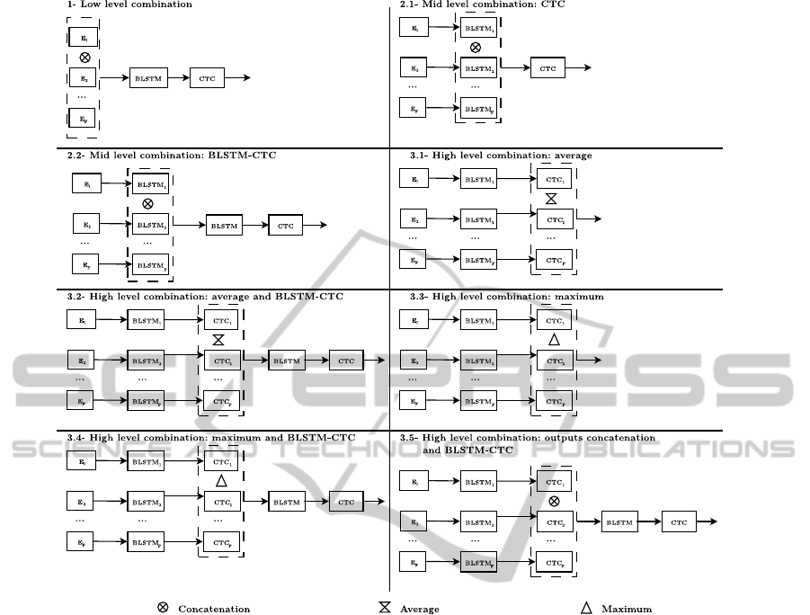
Figure 2: The different BSTM-CTC combinations.

3.3 High Level Combination

Lastly we consider the combination of the CTC out-

puts, a late fusion stage. An ensemble of F BLSTM-

CTC is ﬁrst trained on the F different feature rep-

resentations. The outputs of each BLSTM-CTC are

then combined to form a new output signal. We pro-

pose ﬁve different combination operators for the out-

puts:

1. Averaging outputs: it performs a simple average

of outputs at every instant (Fig. 2 system 3.1).

2. Averaging outputs and training a new BLSTM-

CTC: a BLSTM-CTC is added in order to mea-

sure the ability of the BLSTM-CTC to learn and

correct long term dependencies errors at a charac-

ter level (Fig.2 system 3.2).

3. Combination of outputs and training a new

BLSTM-CTC: this method selects at every instant

the maximum output between the F output labels,

the results are then normalized to appear in the

range [0; 1] (Fig. 2 system 3.3).

4. Selecting the maximum output at all times: this

strategy adds a BLSTM-CTC network on the third

combination, for identical reasons than the second

high level combination (Fig. 2 system 3.4).

5. Selecting the maximum output and training a new

BLSTM-CTC: it is a simple concatenation of the

F CTC outputs at every instant (Fig.2 system 3.5).

Therefore creating a new output representation, if

we consider an alphabet A of size |A|, the new rep-

resentation is of dimension (|A| + 1) × F. This new

output representation is largely superior to the HMM

input dimensions capacity. Hence we use a BLSTM-

CTC to learn and correct errors as well as reduce the

signal dimensionality.

The different combination levels previously pre-

sented all have theoretical advantages and drawbacks.

We now present the experimental results and we ex-

plain why certain combinations outperform the oth-

ers.

BLSTM-CTCCombinationStrategiesforOff-lineHandwritingRecognition

177

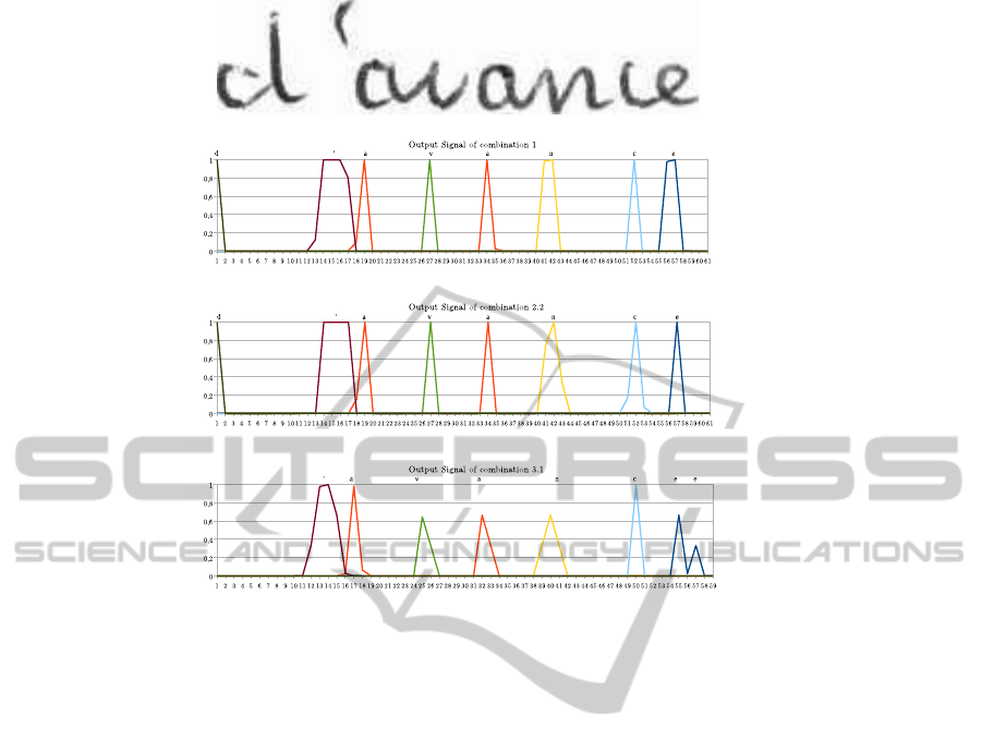
Figure 3: Output signals prior to the HMM on word “d’avance”.

4 EXPERIMENTS

In this section we describe the database and the recog-

nition task we used to compare the various combina-

tion performed on the BLSTM-CTC.

4.1 Database and Task Description

In order to compare our results we use the RIMES

database. This database consists in handwritten letters

addressed to various administrations and registration

services. From these letters, single words were iso-

lated and annotated. The database is divided in three

different subsets: training, validation and test. Each

set contains respectively 44197 images, 7542 images

and 7464 images. The RIMES database was built to

be a low noise database, i.e. the background and fore-

ground pixels are easily identiﬁable. However, the in-

traword variation is very important since 1300 differ-

ent writers participated for writing the letters. The

word length distribution among the three sets is very

similar. It has to be stressed that the words with three

and less characters contribute to more than 40% of

the database. This will affect the HMM lexicon cor-

rection since it is harder to correct short words.

We compare our results on the ICDAR 2009 WR2

task (Grosicki and Abed, 2009). This task consists

in ﬁnding the correct transcription of a word using a

lexicon of 1600 words. The measure used is the Word

Error Rate (WER) on the Top 1 outputs and Top 10

outputs.

In order to learn the system we use the whole

training database to train each part of the system.

This may cause some overﬁtting, however splitting

the training base in order to train each system on sep-

arate bases causes some global loss on the learning

performances.

4.2 Results

We now present the results of the various combina-

tion schemes on the RIMES database for BLSTM-

CTC feature combination. Table 1 presents the results

of the different combinations by displaying the top 1

and top 10 Word Error Rate (WER). We also provide

the raw WER output of the last CTC layer prior to

the HMM layer, i.e. the system without the lexicon

decoding. Combination 3.2 an 3.5 do not outperform

the single features, all other prove to be better strate-

gies than single feature combination.

The best combination is the low level feature com-

bination. The reason is that the BLSTM-CTC is able

to model very efﬁciently the data. In a very similar

fashion to deep neural networks, it models very well

ICPRAM2015-InternationalConferenceonPatternRecognitionApplicationsandMethods

178

Table 1: Results of the different BLSTM-CTC combination experiments on the RIMES database using Word Error Rate.

System Raw WER Top 1 WER Top 10 WER

Single features:

Pixels 41.95 13.19 3.97

SPF 42.23 13.06 4.34

HOG 37.62 12.49 4.47

1-Low Level combination 32.04 9.53 3.01

2-Mid level combinations:

2.1-Output combination and CTC 33.16 10.06 3.11

2.2-Output combination and BLSTM-CTC 32.89 9.6 2.29

3-High Level combinations:

3.1-Averaging 56.8 10.92 2.35

3.2-Averaging and BLSTM-CTC 34.21 13.36 5.68

3.3-Maximum 74.44 12.09 2.93

3.4-Maximum and BLSTM-CTC 34,25 12.45 4.19

3.5-Output combination and BLSTM-CTC 35.73 15.53 6.36

the spatial and time domain dependencies of features.

In order to combine several features using a BLSTM-

CTC it is therefore preferable to directly combine the

features.

Compared to the results produced in (Grosicki and

Abed, 2009) our system is under the performances

of the TUM system based on BLSTM-CTC which

achieves on the same task a 6.83% WER on top 1

and 1.05% WER on top 10. We must point out the

fact that we did very few optimization steps on the

different neural network systems as well as the dif-

ferent preprocessing parameters. The results could be

improved further thanks to a comprehensive research

on the different parameters.

The results of the mid level combinations are in-

teresting since even without relearning the BLSTM

layer used to extract features we obtain a system

that is close to the low level features performance on

Top 1 and outperforms it on Top 10. Relearning the

BLSTMs used as feature extractors may enable fur-

ther improvements of these results.

The outcome of the high level combinations is

more contrasted. On the one hand averaging and max-

imum enable to improve the Top 1 results. On the

other hand relearning a BLSTM-CTC from these out-

puts does not enable further correction, it slightly de-

creases the performances. For system 3.2 it degrades

the system to the point it is worse than the single fea-

ture systems.

It is noteworthy to point out that the Top 10 of sys-

tem 3.1 is better than system 1, hence the averaging

process is able to produce more hypothesis to be used

during the lexicon directed decoding stage. As it can

be seen on ﬁgure 3 the signals between the low level

combination and the averaging are different. The av-

eraging has less peaks achieving the maximum output

value on characters, hence it puts forward more char-

acters that can help explore different paths during the

lexicon directed decoding.

As a ﬁnal note it is interesting to see that relearn-

ing long term dependencies using a BLSTM-CTC for

high level combinations decreases the performance of

the system. This is probably due to the very peaked

output of the BLSTM-CTC. Indeed relearning from

the output probabilities of the BLSTM-CTC were

strong hypothesis are put forward does not enable the

most likely hypothesis to emerge. The BLSTM-CTC

carrying out the combination may simply be over-

learning the data.

5 CONCLUSION

In this paper we presented different strategies to com-

bine feature representations using a BLSTM-CTC.

The best result is achieved using a low level feature

combination (early integration), indeed the internal

spatial and time modeling ability of the BLSTM net-

work is very efﬁcient. The mid level combination

and the high level combination by averaging improve

signiﬁcantly the results of the baseline systems. Fu-

ture work will investigate the importance of retrain-

ing the BLSTMs used as feature extractors for the

mid level features. Retraining these weights may im-

prove further the recognition rate of systems 2.1 and

2.2. We will also investigate the addition of high di-

mension feature extractor. Indeed adding too many

features may lead to a saturation of a single BLSTM-

CTC using the low level strategy, hence training mul-

tiple BLSTM layers with low dimensional inputs may

prove a better solution than working with high dimen-

sional input. Future work may also investigate the

BLSTM-CTCCombinationStrategiesforOff-lineHandwritingRecognition

179

combination of combinations.

REFERENCES

Ait-Mohand, K., Paquet, T., and Ragot, N. (2014). Combin-

ing structure and parameter adaptation of HMMs for

printed text recognition. IEEE Transactions on Pat-

tern Analysis and Machine Intelligence, (99).

Bengio, Y. (2009). Learning Deep Architectures for AI.

Foundations and Trends in Machine Learning, 2(1):1–

127.

Bengio, Y., De Mori, R., Flammia, G., and Kompe, R.

(1992). Global optimization of a neural network-

hidden Markov model hybrid. IEEE Transactions on

Neural Networks, 3(2):252–259.

Bishop, C. M. (1995). Neural networks for pattern recog-

nition. Oxford University Press.

Bunke, H., Bengio, S., and Vinciarelli, A. (2004). Ofﬂine

recognition of unconstrained handwritten texts using

HMMs and statistical language models. IEEE Trans-

actions on Pattern Analysis and Machine Intelligence,

26(6):709–720.

Dalal, N. and Triggs, B. (2005). Histograms of Oriented

Gradients for Human Detection. IEEE Computer

Society Conference on Computer Vision and Pattern

Recognition, 1:886–893.

El-Yacoubi, A., Bertille, J., and Gilloux, M. (1995). Con-

joined location and recognition of street names within

a postal address delivery line. Proceedings of the

Third International Conference on Document Analy-

sis and Recognition, 2:1024–1027.

El-Yacoubi, A., Gilloux, M., Sabourin, R., and Suen, C. Y.

(1999). An HMM-based approach for off-line uncon-

strained handwritten word modeling and recognition.

IEEE Transactions on Pattern Analysis and Machine

Intelligence, 21(8):752–760.

Gehler, P. and Nowozin, S. (2009). On feature combina-

tion for multiclass object classiﬁcation. In IEEE Inter-

national Conference on Computer Vision, pages 221–

228. IEEE.

Gers, F. A. and Schraudolph, N. N. (2002). Learning Pre-

cise Timing with LSTM Recurrent Networks. Journal

of Machine Learning Research, 3:115–143.

Graves, A. (2008). Supervised sequence labelling with re-

current neural networks. PhD thesis.

Graves, A. and Gomez, F. (2006). Connectionist temporal

classiﬁcation: Labelling unsegmented sequence data

with recurrent neural networks. In Proceedings of the

23rd International Conference on Machine Learning.

Graves, A., Liwicki, M., Bunke, H., Santiago, F., and

Schmidhuber, J. (2008). Unconstrained on-line hand-

writing recognition with recurrent neural networks.

Advances in Neural Information Processing Systems,

20:1–8.

Graves, A., Liwicki, M., Fern

andez, S., Bertolami, R.,

Bunke, H., and Schmidhuber, J. (2009). A novel

connectionist system for unconstrained handwriting

recognition. IEEE Transactions on Pattern Analysis

and Machine Intelligence, 31(5):855–68.

Grosicki, E. and Abed, H. E. (2009). ICDAR 2009 Hand-

writing Recognition Competition. In 10th Interational

Conference on Document Analysis and Recognition,

pages 1398–1402.

Hochreiter, S. and Schmidhuber, J. (1997). Long short-term

memory. Neural Computation, 9(8):1735–1780.

Knerr, S., Anisimov, V., Barret, O., Gorski, N., Price, D.,

and Simon, J. (1997). The A2iA intercheque sys-

tem: courtesy amount and legal amount recognition

for French checks. International journal of pattern

recognition and artiﬁcial intelligence, 11(4):505–548.

Kundu, A., He, Y., and Bahl, P. (1988). Recognition

of handwritten word: ﬁrst and second order hidden

Markov model based approach. Computer Vision and

Pattern Recognition, 22(3):457–462.

Lee, A., Kawahara, T., and Shikano, K. (2001). Julius an

Open Source Real-Time Large Vocabulary Recogni-

tion Engine. In Eurospeech, pages 1691–1694.

Menasri, F., Louradour, J., Bianne-Bernard, A., and Ker-

morvant, C. (2012). The A2iA French handwriting

recognition system at the Rimes-ICDAR2011 compe-

tition. Society of Photo-Optical Instrumentation En-

gineers, 8297:51.

Povey, D., Ghoshal, A., Boulianne, G., Burget, L., Glem-

bek, O., Goel, N., Hannemann, M., Motlicek, P., Qian,

Y., Schwarz, P., Silovsky, J., Stemmer, G., and Vesely,

K. (2011). The kaldi speech recognition toolkit. In

IEEE workshop on Automatic Speech Recognition and

Understanding, pages 1–4.

Rabiner, L. (1989). A tutorial on hidden Markov models

and selected applications in speech recognition. Pro-

ceedings of the IEEE, 77(2):257–286.

Vincent, P., Larochelle, H., Yoshua, B., and Manzagol,

P. A. (2008). Extracting and composing robust fea-

tures with denoising autoencoders. In Proceedings of

the Twenty-ﬁfth International Conference on Machine

Learning, number July, pages 1096–1103.

Vinciarelli, A. (2002). A survey on off-line cursive word

recognition. Pattern recognition, 35(7):1433–1446.

Vinciarelli, A. and Luettin, J. (2001). A new normaliza-

tion technique for cursive handwritten words. Pattern

Recognition Letters, 22(9):1043–1050.

Werbos, P. J. (1990). Backpropagation through time: What

it does and how to do it. Proceedings of the IEEE,

78(10):1550—-1560.

Young, S., Evermann, G., Gales, M., Hain, T., Kershaw, D.,

Moore, G., Odell, J., Ollason, D., Povey, D., Valtchev,

V., and Woodland, P. (2006). The HTK book.

ICPRAM2015-InternationalConferenceonPatternRecognitionApplicationsandMethods

180