Modeling Genetical Data with Forests of Latent Trees for Applications in

Association Genetics at a Large Scale

Which Clustering Method should Be Chosen?

D.-T. Phan

, P. Leray

and C. Sinoquet

LINA / UMR CNRS 6241, Polytech/ University of Nantes, rue Christian Pauc, BP 50609, 44306 Nantes, France

LINA / UMR CNRS 6241, Faculty of Sciences, University of Nantes, 2 rue de la Houssini`ere, 44322 Nantes, France

Keywords:

Linkage Disequilibrium, Genome-wide Association Study, Multilocus Association Study, Data Dimension

Reduction, Probabilistic Graphical Model, Bayesian Network.

Abstract:

Association genetics, and in particular genome-wide association studies (GWASs), aim at elucidating the

etiology of complex genetic diseases. In the domain of association genetics, machine learning provides an

appealing alternative framework to standard statistical approaches. Pioneering works (Mourad et al., 2011)

have proposed the forest of latent trees (FLTM) to model genetical data at the genome scale. The FLTM is a

hierarchical Bayesian network with latent variables. A key to FLTM construction is the recursive clustering of

variables, in a bottom up subsuming process. In this paper, we study the impact of the choice of the clustering

method to be plugged in the FLTM learning algorithm, in a GWAS context. Using a real GWAS data set

describing 41400 variables for each of 3004 controls and 2005 individuals affected by Crohn’s disease, we

compare the inﬂuence of three clustering methods. Data dimension reduction and ability to split or group

putative causal SNPs in agreement with the underlying biological reality are analyzed. To assess the risk

of missing signiﬁcant association results through subsumption, we also compare the methods through the

corresponding FLTM-driven GWASs. In the GWAS context and in this framework, the choice of the clustering

method does not impact the satisfying performance of the downstream application, both in power and detection

of false positive associations.

1 INTRODUCTION

With the ﬁnalization of the Human Genome Project

in 2003, it was conﬁrmed that any two individuals

share, on average, 99.9% of their genome with one

another. It is then the sole 0.1% genetic variations that

may explain why individuals are physically different

or should inherit a greater risk of contracting genetic

disorders, such as coronary heart disease, diabetes,

autism, some cancers. As a consequence, identify-

ing the genetic factors underlying these diseases po-

tentially plays a crucial role in prediction, monitoring

subjects with risks, as well as developing new treat-

ments. Deciphering the putative causes of complex

genetic diseases has been one of the main focuses of

human genetics research during the last thirty years.

Among different approaches that have been proposed,

association studies stand out as one of the most suc-

cessful paths, even though their potential is yet to be

fully tapped.

The HapMap Project (Gibbs et al., 2003) and

its successor, the 1000 Genomes Project (The 1000

Genomes Project Consortium, 2010), were launched

with the hope to establish a catalogue of human

genome regions in which people of different popula-

tions have differences.

When no clue is available about the genome re-

gions likely to contain one of the putative causes for

a studied disease, geneticists are compelled to resort

to genome-wide association studies (GWASs). Ge-

netic markers are used for this purpose, as well as

a population of affected and unaffected individuals.

Genetic markers represent as many DNA sequences,

spread over the whole genome, with a known loca-

tion, where the DNA variations within a given popu-

lation may be observed. In a nutshell, GWASs seek

to identify genetic markers whose variants vary sys-

tematically between affected (cases) and unaffected

(controls) individuals (Balding, 2006). The standard

GWAS consists in comparing variant frequencies in

cases and controls, on massive genotypic datasets

(tens of thousands of individuals each described by

Phan D., Leray P. and Sinoquet C..

Modeling Genetical Data with Forests of Latent Trees for Applications in Association Genetics at a Large Scale - Which Clustering Method should Be

Chosen?.

DOI: 10.5220/0005179800050016

In Proceedings of the International Conference on Bioinformatics Models, Methods and Algorithms (BIOINFORMATICS-2015), pages 5-16

ISBN: 978-989-758-070-3

 2015 SCITEPRESS (Science and Technology Publications, Lda.)

hundreds of thousands up to a few millions of ge-

netic markers). The goal is to identify the loci on

the genome for which the distributions of variants are

signiﬁcantly different between cases and controls, us-

ing dependence - namely association - tests (e.g. the

Chi

test). The unit variants, called single nucleotide

polymorphisms (SNPs), which refer to single base

pair changes in the DNA sequence, represent the most

abundant type of variants in human; they are very of-

ten used as markers in GWASs.

The key to GWASs lies in this interesting phe-

nomenon known as ”linkage disequilibrium” (LD)

where variants for different SNPs tend to co-occur

non-randomly (Pritchard and Przeworski, 2001) (the

corresponding SNPs are said to be in LD). The case

would be exceptional if a genetic marker, which is

observed in the population, coincided with a genetic

causal factor. Nevertheless, thanks to LD, a depen-

dence exists between the non observed causal factor

and a genetic marker nearby the former. On the other

hand, by deﬁnition, a dependence exists between the

causal factor and the disease of interest. Therefore, it

is likely that a dependence will be detected between

the nearby genetic marker and the disease.

In the human genome, the HapMap project con-

ﬁrmed evidence of the linkage disequilibrium, this la-

tent structure organized in the so-called ”haplotype

blocks”. Therein, regions showing high dependences

between contiguous markers (blocks) alternate with

shorter regions characterized by low statistical depen-

dences. In general, LD exhibited among physically

close loci is stronger than LD between SNPs that are

farther apart. In other words, LD decays with dis-

tance.

However, standard GWASs do not fully exploit

LD. Some authors proposed to test combinations of

SNPs - haplotype blocks - against the disease, rather

than merely each SNP against the disease: this is the

principle of multilocus approaches. First, if the causal

SNP has low frequency and is not in high LD with

any one of the genotyped SNPs, then the multilocus

test will tend to be more powerful. Besides, the ad-

vantage to the GWAS is that the LD is likely to reveal

an excess of haplotype sharing around a causative lo-

cus, amongst cases. Third, testing haplotypes instead

of SNPs is a way to implement data dimension re-

duction. In this context, ﬁne LD modeling at genome

scale is required.

Few works have focused on LD modeling at

genome scale, which is a challenging task. The pro-

posals of (Abel and Thomas, 2011) and (Verzilli et al.,

2006) both rely on the use of Markov random ﬁelds,

a popular kind of probabilistic graphical models. Two

scalable models designed for the speciﬁc purpose of

multilocus GWASs have been described by (Brown-

ing and Browning, 2007) and (Mourad et al., 2011).

The approach in (Browning and Browning, 2007) re-

lies on a variable length Markov chain (VLMC), a

Markov model where the size of the memory con-

ditioning the prediction of the variant at a given lo-

cation is ﬂexible. In contrast with this block-based

method, the works in (Mourad et al., 2011) seek to

subsume clusters of SNPs through latent variables.

SNPs within the same cluster are not necessarily con-

tiguous. Such latent variables are intented to be tested

against the disease. Both methods account for the

fuzzy nature of LD since block boundaries are not ac-

curately deﬁned over the genome. However, being

blocked-based, the method in (Browning and Brown-

ing, 2007) cannot take into account long-range depen-

dences. Moreover, LD is intrinsically hierarchical,

with clusters of SNPs recursively structured in clus-

ters of lower and lower correlated SNPs. To attempt

a faithful representation of LD upstream of a GWAS,

hierarchical clustering is one of the key ingredients of

the learning algorithm of the Bayesian model used in

(Mourad et al., 2011). Since clustering is central to

learning the model in (Mourad et al., 2011), namely

the forest of latent tree models (FLTM), this paper

analyses the impact of the choice of the clustering

method in a GWAS context.

2 OBJECTIVES AND

ORGANIZATION OF THE

PAPER

In the remainder of this paper, data partitioning - or

clustering - denotes the generation of a set of non

overlapping clusters. Such a task is highly complex.

Though, choosing a clustering method to learn an

FLTM must comply with the scalability goal. This

paper compares the native clustering method used in

(Mourad et al., 2011) (CAST

bin

) with a relaxed ver-

sion (CAST

real

) and another clustering method (DB-

SCAN). In this framework, two aims of the paper are

to evaluate whether FLTM learning is robust to the

choice of the clustering method and how close a clus-

tering method approximates the underlying biological

reality. To fulﬁll the ﬁrst goal, a protocol is used that

relies on assessing how much two partitions agree.

The second objective is met by applying the previ-

ous protocol to compare each clustering method to a

reference partition supposed to be close to biological

reality. The Haploview software program is the tool

chosen to derive such a reference partition. Focusing

on the data dimension reduction aspect, a third objec-

BIOINFORMATICS2015-InternationalConferenceonBioinformaticsModels,MethodsandAlgorithms

tive of the paper is to analyze the impact of the choice

of the clustering method on data subsumption quality.

By construction, an FLTM-based GWAS processes

data subsumed through latent variables, to hopefully

pinpoint the interesting regions of a genome without

testing each SNP for association. Thus, the third ob-

jective of this paper is to assess whether the choice

of the clustering method impacts the risk of missing

signiﬁcant association results through subsumption.

FLTM-driven GWASs are run to study this impact.

The remainder of the paper is organized in ﬁve

sections. Section 3 ﬁrst offers a brief introduction to

Bayesian networks, the kind of probabilistic graphi-

cal models FLTM is based upon. Then section 3 pro-

vides a broad brush description of the FLTM learning

algorithm together with a sketch of a GWAS strat-

egy based on FLTM. Section 4 brieﬂy refers to the

native clustering method used in FLTM (CAST

bin

)

and to its relaxed version (CAST

real

); it then moti-

vates the choice of the alternative clustering method

(DBSCAN) plugged in the FLTM learning algorithm.

Then, section 5 explains the design of the protocols

and methods used in our work. First, we discuss

the protocol used to assess how much two partitions

agree. Second, we justify the use of the Haploview

software program to derive the reference partition,

supposedly the closest representation of the underly-

ing reality. In section 6, we describe the Crohn’s dis-

ease GWAS data used in our study. Section 7 is de-

voted to the presentation and discussion of the results

observed.

3 FRAMEWORK AND FLTM

MODEL

The FLTM model is a tree-structured Bayesian net-

work (BN). Therefore this section ﬁrst brieﬂy in-

troduces Bayesian networks, to further focus on the

FLTM model. The principle of the FLTM learning

algorithm is then presented. Finally, the principle

for a multilocus GWAS based on the FLTM model

is sketched.

3.1 A Brief Reminder about

Probabilistic Graphical Models

When probabilistic graphical models are learnt from

scratch, one has to learn their two fundamental com-

ponents from a data matrix. In this matrix, the lines

correspond to the observations and the columns cor-

respond to the variables X

(1 ≤ i ≤ n). For exam-

ple, in the case of genetical data, the observations

(a) (b) (c)

Figure 1: (a) Latent tree model (LTM). (b) Forest of la-

tent tree model (FLTM). (c) Latent class model. Observed

and latent variables are represented in dark and light color

shades, respectively.

are the individuals (cases and controls) in the popu-

lation studied, and the variables are the SNPs. The

qualitative component of a BN is a graph where the

variables are represented as nodes. The connections

between the nodes represent the direct dependences

between the variables. More speciﬁcally, the qualita-

tive component of a BN is a directed acyclic graph.

The quantitative component of a BN is a collection of

probability distributions, denoted as ”the parameters

θ”. If the variable X

has no parent in the graph, then

is merely an a priori distribution (θ

= P(X

)). If

the variable X

has a set of parents Pa

, then θ

is the

conditional distribution θ

= P(X

| Pa

). In particu-

lar, Bayesian networks offer a practicable framework:

exploiting the network structure, this framework al-

lows to compute the joint probability of the variables,

P(X), as a product of low-dimensional functions.

It may happen that the data observed is thought to

embed a latent structure, depicted through latent vari-

ables and their connections in the learnt BN. In this

case, learning the Bayesian network encompasses the

task of inferring the latent variables, and their connec-

tions within the BN.

The FLTM model is a forest of latent tree models

(LTMs). The Figure 1(a) shows that an LTM is char-

acterized by a hierarchical structure organized in lay-

ers. The ﬁrst layer is composed of the observed vari-

ables. The other layers are composed of latent vari-

ables. The learning algorithm of the FLTM (see Fig-

ure 1(b)) relies on the simplest LTM that may be de-

scribed, the latent class model (LCM). A latent class

model connects a single latent variable to child vari-

ables ; no connections are allowed between the latter

(see Figure 1(c)).

3.2 Sketch of the FLTM Learning

Algorithm

Learning a BN is a hard task that consists in inferring

both the graph structure and the parameters. Learn-

ing a BN with latent variables is far more compli-

cated. First, one does not even know how many latent

ModelingGeneticalDatawithForestsofLatentTreesforApplicationsinAssociationGeneticsataLargeScale-Which

ClusteringMethodshouldBeChosen?

variables have to be inferred. Second, in a BN with-

out latent variables, the parameters are estimated to

maximize the likelihood, that is the probability of the

(observed) data given the parameters. In contrast to

this rapid algorithm, a slow procedure has to be em-

ployed for BNs with latent variables, the expectation-

maximization algorithmdedicated to learn parameters

in the case of missing data. Prior knowledge (the hi-

erarchical LD structure) is used by the speciﬁc pro-

cedure described in (Mourad et al., 2011), to provide

a scalable learning algorithm. Figure 2 depicts the

principle of this iterative algorithm, based on an as-

cending hierarchical clustering procedure.

Figure 2: Sketch of the iterative FLTM learning algorithm.

In the case of LD modeling, the observed variables

are the SNPs. The cardinality of these observed vari-

ables is equal to 3, which codes for minor homozy-

gosity, heterozygosity and major homozygosity. The

ﬁrst iteration starts with the partitioning of the ob-

served variables into non overlapping clusters of pair-

wise highly dependent SNPs. No two variables are

allowed in the same cluster if their physical distance

on the genome is above a given threshold, δ. For each

cluster, an LCM is constructed whose child variables

are the variables in the cluster and whose latent vari-

able is created. The approach of (Mourad et al., 2011)

considers discrete latent variables whose cardinalities

may be different from one another; a heuristic is used

to determine the speciﬁc cardinality of each latent

variable. This speciﬁc cardinality is computed as an

afﬁne function of the number of variables in the clus-

ter. Then, the parameters of each LCM are estimated

through the standard expectation-maximization pro-

cedure. Knowing the parameters of each LCM fur-

ther allows to impute the data corresponding to its la-

tent variable. Such imputed data are used by a val-

idation step; this step relies on a normalized mutual

information criterion to examine whether each novel

latent variable is sufﬁciently informative to subsume

its child variables. The data is updated with the val-

idated latent variables replacing their child variables.

The validated latent variables can thus be considered

as observed variables and an iteration begins anew.

This ascending process is iterated until no valid

cluster can be identiﬁed, or a single cluster of maxi-

mal size is obtained. Among other parameters of the

learning procedure, the clustering procedure plugged

in the algorithm is likely to impact the quality of the

LD modeling, and therefore the quality of the GWAS

performed downstream.

3.3 Performing a GWAS Guided by the

FLTM Model

Central to the use of the FLTM model for a GWAS

purpose are the request for data dimension reduction

and the motivation for a multilocus strategy. In the

study described here, we have implemented a multi-

locus GWAS strategy as follows: in the lowest lay-

ers, we traverse the forest top down, following a best-

ﬁrst search strategy which only tests all child nodes

for the nodes whose association signiﬁcances (i.e. p-

values) are below a threshold. The way to compute

this threshold is speciﬁc to the layer the variable be-

longs to. These child nodes are selected in turn with

respect to the appropriate threshold. The standard

Chi

test is applied to test a variable against the dis-

ease and to provide a pointwise p-value. We now

explain how to compute the thresholds for the vari-

ables in the lowest layers. To test statistical signiﬁ-

cance, we consider a global threshold, say α = 5%.

The pointwise p-value of a variable is corrected based

on permutations applied on all the variables in this

variable’s latent layer. Thus, the correction is layer

speciﬁc. Statistical signiﬁcance is assessed by testing

the condition (p-value

corrected

≤ α). The details and

justiﬁcation for this correction will be provided in an

extended version of the article. On the other hand,

due to dimension reduction, the highest layers have a

low number of variables. No correction is applied for

these layers, from which we systematically select the

top most associated variables (e.g. β = 10%).

BIOINFORMATICS2015-InternationalConferenceonBioinformaticsModels,MethodsandAlgorithms

4 THE CAST AND DBSCAN

PARTITIONING METHODS

Performing an optimal clustering is NP-hard (Ack-

erman and Ben-David, 2009). Therefore, heuristics

must be designed instead. In this paper, we focus

on two partitioning methods, CAST and DBSCAN,

to study how they impact LD modeling and a further

downstream GWAS analysis.

Since we address high-dimensionaldata, we could

not envisage the use of ascending hierarchical cluster-

ing, whose complexity scales in O(n

) where n is the

number of objects to be asssigned to clusters. More-

over, in contrast to AHC and k-means, another well

known partitioning method, CAST and DBSCAN do

not request the tuning of the number of clusters.

Partitioning objects into clusters relies on pairwise

distances (alternatively pairwise similarities). Stor-

ing a pairwise similarity matrix at the genome scale

is intractable. Thus, following (Mourad et al., 2011),

we acknowledge a physical constraint, δ, expressed in

kbp (kilobase pairs), in both implementations of the

CAST and DBSCAN methods. This constraint δ rep-

resents the physical distance on the genome beyond

which two objects (in our case two variables) are not

allowed in the same cluster. Additional calculus is re-

quired to estimate the distance between two variables

one of which at least is a latent variable.

The CAST (Cluster Afﬁnity Search Technique) al-

gorithm was proposed in (Ben-Dor et al., 1999) and

is depicted in (Cahill, 2002). Its theoretical runtime

complexity scales in O(n

(log(n))

), with c some

constant, and its empirical complexity allows to han-

dle high-dimensional data. CAST is the native clus-

tering method used in the FLTM learning algorithm

depicted in (Mourad et al., 2011).

To decide cluster membership, CAST relies on

an afﬁnity measure. In the implementation of CAST

adapted to FLTM learning, the binary similarity mea-

sure is assessed as the thresholded mutual informa-

tion (MI). A parameter q

pairwise

(e.g. 50%) allows

to compute the MI quantile (e.g. median) over the

pairs of variables whose physical distance is below

δ. This quantile allows to assign a binary similar-

ity (0/1), as in the native FLTM learning algorithm.

In this study, we also consider the unthresholded ver-

sion. These two CAST versions are denoted CAST

bin

and CAST

real

The DBSCAN (Density-Based Spatial Clustering

of Applications with Noise) algorithm was proposed

in (Ester et al., 1996). Its theoretical runtime com-

plexity is O(n

), where n is the number of objects

to be assigned to clusters. However, its empirical

complexity is known to be lower. To grow clusters,

DBSCAN relies on the merging of objects’ neighbor-

hoods. This method requires two parameters: R, the

maximum radius of the neighborhood to be consid-

ered, and N

min

, the minimum number of neighbors

needed for a cluster.

We have chosen DBSCAN as it is resistant to

noise. Besides, DBSCAN is known to be able to iden-

tify a cluster embedded in another cluster. On the

genome line, long-range LD corresponds to this sit-

uation.

5 METHODS

In this section, we ﬁrst present the protocol used to

evaluate how much two partitions agree when fo-

cusing on the top most associated SNPs found by a

GWAS. Then, we motivate how we derived the so-

called reference partition (to be further deﬁned). This

methodological section ends with the presentation of

the protocol used to compare the impact of the choice

of the partitioning method on the subsequent GWAS.

For this purpose, we rely on GWAS results published

in the literature.

5.1 Comparing Two Partitions

To cope with the genome scale, we were compelled to

select a simple method: we focused on the compari-

son of the partitions respectively obtained for the ﬁrst

layer (SNPs) by two partitioning methods, and we ex-

amined how the top most associated SNPs identiﬁed

by a GWAS are distributed among the clusters.

The methods dedicated to the comparison of two

partitions may be categorized into three main groups

(Meila, 2005). Two groups attempt to map a partition

onto the other, either from set matching functions, or

from information theory-centered methods. The third

category relies on counting for how many pairs of el-

ements two partitions agree or disagree. The FLTM-

driven GWAS strategy is a multilocus strategy by def-

inition. In this multilocus GWAS framework, it is rel-

evant to analyze pair agreement between two parti-

tioning methods, for a selection of top most associ-

ated SNPs. A counting method ﬁts well this purpose

of focusing on a subset of SNPs.

Given two partitions over the same set of objects,

and a pair of objects (in our case, a pair of variables),

an agreement means that the two partitions both group

the two variables in a cluster or both assign two differ-

ent clusters to the two variables. Given two partitions

and P

, let

• N

, the number of pairs both partitions assign to

one cluster,

ModelingGeneticalDatawithForestsofLatentTreesforApplicationsinAssociationGeneticsataLargeScale-Which

ClusteringMethodshouldBeChosen?

• N

, the number of pairs both partitions assign to

different clusters,

• N

, the number of pairs kept in the same cluster

by P

but splitted by P

• N

, the symmetric case of the latter.

From here, a large set of comparison measures is

available. We selected three measures to perform the

following comparisons: CAST

bin

versus CAST

real

CAST

bin

versus DBSCAN, CAST

real

versus DB-

SCAN, and each of the three methods CAST

bin

CAST

real

and DBSCAN versus the reference parti-

tion (to be deﬁned in section 5.2). The comparison

measures selected are:

• the Rand index (Rand, 1971):

RI =

+ N

(1)

for which we used instead an adjusted corrected-

for-chance version (ARI =

RI−expected RI

maximum RI−expected RI

)

(for the detailed description, see (Hubert and Ara-

bie, 1985));

• the Mirkin distance (Mirkin, 1998):

MI =

+ S

− 2S

(2)

with

∑

cluster

∈P

| cluster

, j = 1, 2

∑

cluster

∈P

, cluster

∈P

| cluster

| | cluster

and n the number of objects to be assigned to clus-

ters and | S | the size of set S;

• the Fowlkes-Mallows index (Fowlkes and Mal-

lows, 1983):

FM =

+ N

. (3)

5.2 Deriving the Reference Partition

The reference partition intends to be the closest rep-

resentation of the underlying reality, that is the hap-

lotype blocks. We used the Haploview software pro-

gram (Gabriel et al., 2002) for this purpose. This ap-

plication allows to select commonly used block deﬁ-

nitions to partition the genome into regions of strong

LD (Gabriel et al., 2002; Wang et al., 2002). As this

block generation is dedicated to handle genetical data,

Haploview can only be used for the ﬁrst layer (ob-

served variables). This reason explains why the parti-

tioning method of the Haploview application has not

been plugged in the FLTM learning algorithm.

6 CROHN’S DISEASE GWAS

DATA

The Crohn’s disease data set we used is

made available by the WTCCC Consortium

(http://www.wtccc.org.uk/); it consists of 5009 indi-

viduals genotyped using the Affymetrix GeneChip

500K Mapping Array Set (3004 controls, 2005

cases). We performed the same data quality control

as the WTCCC. We excluded individuals, using

exactly the same criteria as the WTCCC ((WTCCC,

2007), page 26) (e.g. individuals with more than 3%

missing data across all SNPs; individuals sharing

more than 86% of identity with other ones). The rules

to exclude SNPs were also modelled after those of the

WTCCC (e.g. missing rate over 5%; if MAF (minor

allele frequency) under 5%, missing rate threshold

decreased to 1%) ((WTCCC, 2007), page 27).

In this paper, we focus on chromosome 2, known

to harbour SNPs with susceptibility towards Crohn’s

disease. The initial WTCCC data set describes 41400

SNPs. After the quality control step, our data con-

sisted of 38730 SNPs.

7 RESULTS AND DISCUSSION

The parameter t

CAST

(see details in (Cahill, 2002))

speciﬁc to the CAST method, whatever the version

(bin or real), was empirically set to 0.50. The pa-

rameter q

pairwise

speciﬁc to the CAST

bin

clustering

method was empirically chosen to be 50%. The N

min

and R parameters speciﬁc to DBSCAN were tuned to

2 and 0.2 respectively. The FLTM learning algorithm

requires the setting of six parameters. We systemati-

cally evaluated the coefﬁcients of the afﬁne function

used to determine the cardinality of each latent vari-

able, ℓ

and ℓ

, in [0.2, 0.3, 0.4, 0.5] × [1, 2]. We ob-

served no differences between the eight settings, with

regard to the sizes and contents of the clusters. Thus,

ℓ

and ℓ

were set 0.5 and 1. Following (Mourad

et al., 2011), we ﬁxed the maximum cardinality as

20, the physical distance constraint δ as 45 kbp and

the number of restarts of the stochastic expectation-

maximization procedure as 10. The threshold for the

quality control of the candidate latent variables was

set to a low value, 0.01. The GWAS thresholds α and

β were ﬁxed to 5% and 10%. The study was con-

ducted using a 3.3 GHz processor. We had to adapt

the generic versions of the CAST and DBSCAN al-

gorithms, to store a sparse similarity matrix instead

of a pairwise similarity matrix (see section 4).

BIOINFORMATICS2015-InternationalConferenceonBioinformaticsModels,MethodsandAlgorithms

Layer

38730

8241

190

8243

178

6890

0 10000 20000 30000 40000

0 1 2 3

CAST

real

CAST

bin

DBSCAN

Number of variables

5 10 15

0.0 0.2 0.4 0.6 0.8

Number of variables

Density

Haploview

CAST

real

CAST

bin

DBSCAN

(a) (b)

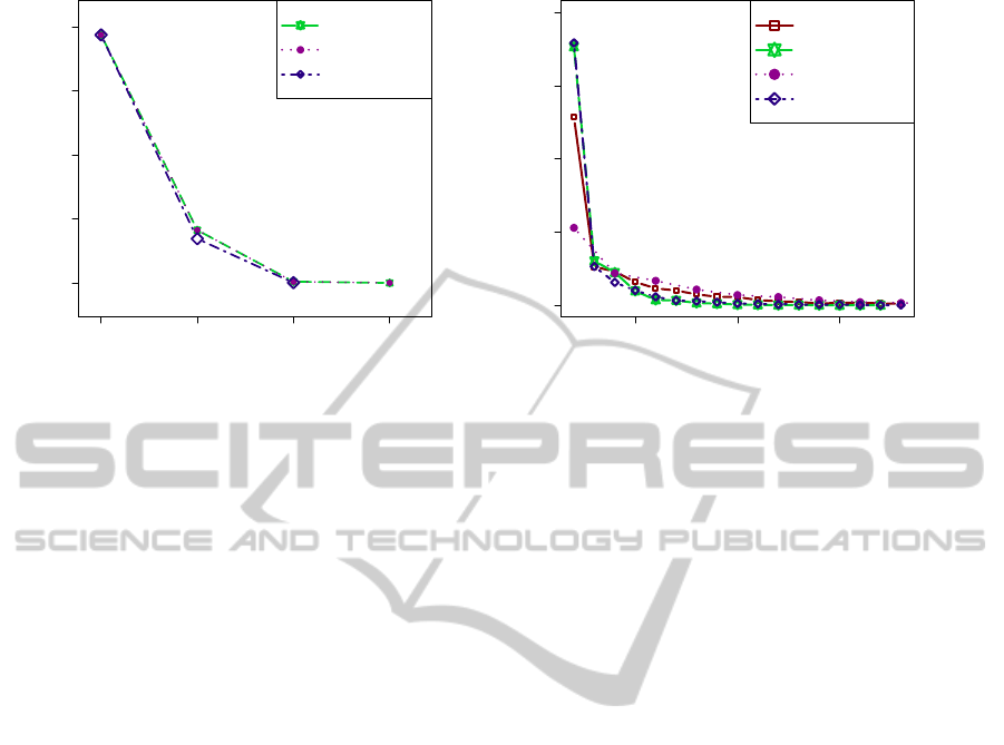
Figure 3: Impact of the choice of the partitioning methods CAST

bin

, CAST

real

and DBSCAN on the structure of the FLTM

model. (a) Impact on the number of variables per layer. (b) Impact on the sizes of the clusters for the ﬁrst layer (observed

layer).

7.1 FLTM Architectures

On average, the running time observed for FLTM

learning with each clustering method is in the order of

60 hours. A closer examination shows that clustering

and other operations only required at most 1 minute

for each layer, and that practically all the running time

was spent in the expectation-maximization procedure

(see section 3.2). Moreover, it is likely that the pres-

ence of a few clusters of large size (size up to 50)

severely increases running times for the expectation-

maximization procedure.

We ﬁrst analyze the impact of the partitioning

method on the structure of the FLTM model con-

structed prior to a GWAS. Figure 3 (a) compares

the impacts of the three partitioning methods on the

data dimension reduction. We observe that for any

layer, the total number of latent variables created us-

ing CAST

real

is always greater than that created using

DBSCAN. Moreover, layer 3 does not exist for DB-

SCAN whereas it exists for CAST

bin

and CAST

real

Indeed, for DBSCAN, no more variables can be

grouped in layer 2: all candidate clusters are sin-

gletons. The numbers of variables in layers 1 and 3

are either very close or similar between CAST

bin

and

CAST

real

. Again, among the three methods, the num-

bers of variables in layer 2 are the closest for CAST

bin

and CAST

real

Figure 3 (b) provides the histogram for the sizes

of the clusters in the ﬁrst (observed) layer, for each

of the three partitioning methods, together with the

histogram of the reference Haploview partitioning. It

has to be mentioned that, for reasons of presentation,

the histograms have been truncated. Very few clus-

ters of large sizes are observed: the maximum sizes

observed are 18, 45 and 50 for CAST

real

, DBSCAN

and CAST

bin

, respectively. Such clusters would nor-

mally appear far apart on the right section of Figure 3

(b).

First, we observe that from size 3, the CAST

bin

curve is slightly above the CAST

real

and DBSCAN

curves. Besides, the latter curves are nearly super-

imposed. Finally, we note that from size 3, the curve

relative to the reference partitioning is located slightly

below that of CAST

bin

, on the one hand, and slightly

abovethe quasi superimposed curves of CAST

real

and

DBSCAN, on the other hand.

Therefore, the general conclusion to draw for

this section is the propensity for DBSCAN to pro-

duce a lower number of variables than CAST

bin

and

CAST

real

, but with no clear impact on the differences

between the cluster size histograms.

7.2 Comparison of the Partitioning

Methods in a GWAS Context

In a GWAS context, we wish to focus in pri-

ority on pairs of SNPs selected among the top

SNPs found most associated with the studied dis-

ease. The standard tool PLINK was used to

identify these top SNPs (Purcell et al., 2007)

(http://pngu.mgh.harvard.edu/purcell/plink/). Rely-

ing on PLINK, we performed a single-SNP GWAS on

the WTCCC data set relative to chromosome 2. The

association test used was the Chi

. We have extended

the agreement analysis of two partitions to embedded

ModelingGeneticalDatawithForestsofLatentTreesforApplicationsinAssociationGeneticsataLargeScale-Which

ClusteringMethodshouldBeChosen?

0 200 400 600 800 1000

0.5 0.6 0.7 0.8 0.9 1.0

Top N Variables

CAST

real

CAST

bin

DBSCAN

Adjusted Rand Index

0 200 400 600 800 1000

0.00 0.02 0.04 0.06 0.08

Top N Variables

CAST

real

CAST

bin

DBSCAN

Mirkin Distance

0 200 400 600 800 1000

0.4 0.5 0.6 0.7 0.8 0.9 1.0

Top N Variables

CAST

real

− CAST

bin

DBSCAN−CAST

bin

DBSCAN−CAST

real

Adjusted Rand Index

(a) (b) (c)

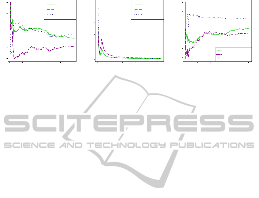
Figure 4: Agreement of two partitioning methods, in a GWAS context. (a) and (b) Agreement of a partitioning method with

the reference block partitioning method used by Haploview. Comparison for the partitioning methods CAST

bin

, CAST

real

and DBSCAN. Impact of the number of top SNPs considered on the agreement. The top SNPs considered are those found

most signiﬁcantly associated by a standard single-SNP GWAS. (a) Adjusted Rand index. (b) Mirkin distance. (c) Pairwise

comparison of the partitioning methods CAST

bin

, CAST

real

and DBSCAN. Impact of the number of top SNPs considered on

the agreement. Adjusted Rand index.

sets of associated SNPs, increasing the size of the set

of top associated SNPs up to 1000.

Figures 4 (a) and (b) compare the partioning meth-

ods CAST

bin

, CAST

real

and DBSCAN together with

Haploview, following two of the three comparison cri-

teria described in section 5.1.

The adjusted Rand index is all the higher as the

agreement between two partitioning methods is high.

Thus, we observe that CAST

bin

does not agree with

the reference (Haploview) partitioning as well as

CAST

real

and DBSCAN. This speciﬁcity of CAST

bin

is explained by the conversionof real mutual informa-

tion values into binary values (see the role of param-

eter q

pairwise

in section 4). This discretization there-

fore entails slightly larger cluster sizes for CAST

bin

as seen in section 7.1.

On the left section of Figure 4 (a), the index

is computed from few top SNPs. We observe that

CAST

bin

and CAST

real

show a high Rand index in

contrast to DBSCAN. However, in a GWAS context,

we do not wish to examine only, say, the 20 top sig-

niﬁcantly associated SNPs. Thus, the most relevant

section to focus on is around 50-100 top SNPs. In

this latter section of Figure 4 (a), we observe that

the CAST

real

and DBSCAN curves are comparatively

close and clearly located higher than the CAST

bin

curve. This trend is observed up to the 1000 top most

associated SNPs.

In Figure 4 (b), a low Mirkin distance indicates

a high agreement between two partitioning meth-

ods. The observations in Figure 4 (b) conﬁrm that

CAST

bin

’s agreement with Haploviewclustering is al-

ways worse than the other two methods’. We have

not shown the results for the Fowlkes-Mallows index

as the curves obtained are quasi superimposable with

those plotted for the adjusted Rand index.

The ﬁrst general conclusion to draw from this ﬁrst

series of agreement comparisons on the Crohn’s dis-

ease data set is that DBSCAN and CAST

real

show

a high level agreement with Haploview partitioning,

both being quite clearly better than CAST

bin

Figure 4 (c) displays the results for pairwise com-

parisons: CAST

real

versus CAST

bin

, DBSCAN ver-

sus CAST

bin

and DBSCAN versus CAST

real

. Ac-

cording to the adjusted Rand index, DBSCAN and

CAST

real

show a high agreement. Given our pre-

vious observations, we expected that CAST

bin

and

CAST

real

would show a low level agreement, which

is conﬁrmed. DBSCAN and CAST

bin

yield partitions

that almost always disagree more than for the two for-

mer couples of partitioning methods. This trend is

conﬁrmed with the Mirkin distance and the Fowlkes-

Mallows index (results not shown).

As a second general conclusion of this section,

we cross-conﬁrm one of our previous observations:

DBSCAN and CAST

real

each show a high agree-

ment with Haploview. This fact is therefore also

reﬂected by a high agreement between DBSCAN and

CAST

real

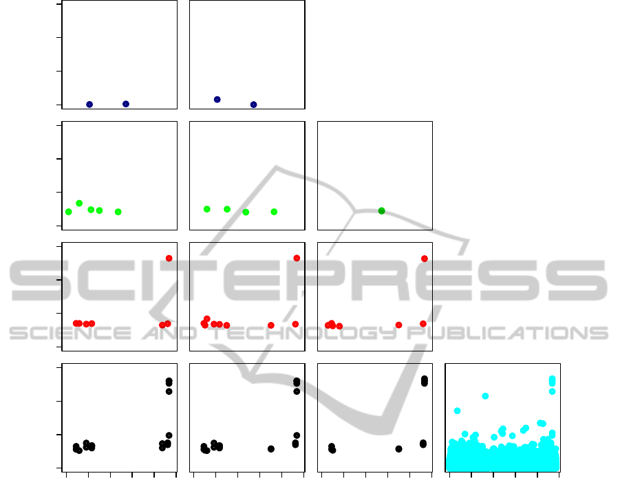
7.3 FLTM-driven GWASs

In Figure 5, the comparison of plots (a) to (c) and

plot (d) shows how the dimension reduction allows

to pinpoint the potentially most interesting regions

on the genome. Thus, ”sparse” association proﬁles

are produced, as opposed to the dense output of the

standard single-SNP GWAS.

The two putative causal SNPs located on chro-

mosome 2 respectively reported in the WTCCC

study (WTCCC, 2007) and in (Barrett et al., 2008)

BIOINFORMATICS2015-InternationalConferenceonBioinformaticsModels,MethodsandAlgorithms

0 5 10 15

(a) CAST

bin

−log

(p−value)

Layer 3

0 5 10 15

−log

(p−value)

Layer 2

0 5 10 15

−log

(p−value)

Layer 1

0 50 100 200

0 5 10 15

−log

(p−value)

Layer 0

Mbp

(b) CAST

real

Layer 3

Layer 2

Layer 1

Layer 0

0 50 100 200

Mbp

Layer 2

Layer 1

Layer 0

0 50 100 200

Mbp

0 50 100 200

(d) Single−SNP GWAS

Mbp

Figure 5: Impact of the choice of the partitioning method on the multilocus GWAS results. For the FLTM-based GWASs ((a)

to (c)), one ”sparse” association proﬁle is displayed for each layer, as not all variables in a layer are examined. The single-SNP

GWAS in (d) was performed using the gold standard PLINK (Purcell et al., 2007). Its output only deals with variables in layer

0 (observed variables). All plots show initial (i.e. non corrected) p-values.

are identiﬁed by the three FLTM-driven GWASs.

Given that we used the same data set as in (WTCCC,

2007), one of the two results was expected. However,

this result was not guaranteed, because of the data

dimension reduction and of the subsumption involved

in an FLTM-driven GWAS. Besides, it must be

highlighted that the study in (Barrett et al., 2008)

analyzed 8059 individuals (3230 cases and 4829

controls), whereas the WTCCC data set describes a

population of size 5009. Table 1 shows that CAST

bin

and CAST

real

capture exactly the same four highly

associated SNPs through the latent variables L

and

, belonging to layer 1. These variables are the

right-most latent variables in layer 1, on the plots (a)

and (b) of Figure 5. The virtual location of a latent

variable is computed as the average of the locations of

its child variables. Thus, the location of L

(or L

) is

233837691 bp. The p-values computed for L

and L

differ since the data imputed for these latent variables

differ. For either CAST

bin

or CAST

real

, the SNP

published in (WTCCC, 2007) is not grouped with

other SNPs into a cluster, in contrast to DBSCAN.

Table 1 shows that for DBSCAN, the latent variable

subsumes SNPs among which are the two already

published putative causal SNPs. L

and L

three highly associated SNPs, including the putative

causal SNP published in (Barrett et al., 2008). The

virtual location of L

is 233830355 bp. We can see

that L

captures LD on a slightly wider range than

, since the regions encompassed by the former and

the latter variables spread over 29292 and 21571 bp,

respectively.

A more thorough analysis of the Affymetrix ar-

ModelingGeneticalDatawithForestsofLatentTreesforApplicationsinAssociationGeneticsataLargeScale-Which

ClusteringMethodshouldBeChosen?

Table 1: Analysis of the latent variables in layer 1 found signiﬁcantly associated with Crohn’s disease, by the three FLTM-

driven GWASs with plug-in CAST

bin

, CAST

real

and DBSCAN, respectively. For each clustering method, the latent variable

is described on the ﬁrst line. On the following lines, the highly associated SNPs subsumed by this latent variable are depicted.

The identiﬁer of each SNP is provided (rsXXXXXXX). The • character highlights the SNPs which are common children of

latent variables L

(or L

) and L

. ∗ Note that the association tests used may differ between studies.

Clustering method Variable Location p-value p-value reported in another study

∗

CAST

bin

latent L

233837691 (1) 5.86× 10

−14

rs6752107 233826187 • (2) 9.65× 10

−14

(3)

rs6431654 233826508 • (2) 9.96× 10

−14

(4)

rs3828309 233845149 • (2) 2.30× 10

−13

(5) 2× 10

−32

(Barrett et al., 2008)

rs3792106 233855479 (2) 3.70× 10

−12

CAST

real

latent L

see (1) 5.52 × 10

−14

see (2)

DBSCAN

latent L

233830355 6.58× 10

−14

rs10210302 233823578 4.60 × 10

−14

7× 10

−14

(WTCCC, 2007)

rs6752107 233826187 • see (3)

rs6431654 233826508 • see (4)

rs3828309 233845149 • see (5) 2× 10

−32

(Barrett et al., 2008)

ray indicates that the region encompassed by L

[233826187, 233855479], contains four highly as-

sociated SNPs, interspersed with three non associ-

ated SNPs. Similarly, the interval covered by L

[233823578, 233845149], contains eight SNPs, in-

cluding four non associated SNPs. Clearly, among

the four highly associated SNPs pinpointed by each

of L

and L

, respectively three and two SNPs are

highly associated with the disease because they are

in LD with a putative causal SNP (see Table 1). How-

ever, not every SNP close to a putative causal SNP

has been incorporated in the cluster subsumed by L

or L

. To conﬁrm the relevance of the clustering

performed, an in-depth examination shows that these

former close SNPs that are not in LD with putative

causal SNPs are found poorly associated with the dis-

ease (in the order of 10

−1

). Importantly,even the SNP

ﬂanking on the left the causal putative SNP published

in (Barrett et al., 2008) and having a p-value equal to

1.32 × 10

−5

, was not retained in L

or L

’s cluster.

This observation shows that a ﬁne-grain clustering is

achieved for each of the three partitioning methods.

Therefore, a ﬁrst remarkable result is that the sub-

sumption process does not hinder the informative-

ness of L

, L

and L

: L

, L

and L

are still found

highly associated with the disease (5,86 × 10

−14

5,52 × 10

−14

, 6.58× 10

−14

respectively).

Moreover, a second remarkable result is ob-

tained. The standard GWAS (Figure 5 (d)) iden-

tiﬁes two SNPs with a high statistical signiﬁ-

cance (rs13394205, located at around 18 Mbp

(17849508), and rs11887827, located at around 81

Mbp (81519665)). The p-values of these two

SNPs are respectively 2.28× 10

−9

and 1.81× 10

−11

None of these SNPs were reported in former stud-

ies (WTCCC, 2007) and (Barrett et al., 2008), which

identiﬁed them as false positives. In the layers 0 of

the plots (a) to (c) of Figure 5, none of these two

SNPs either appears. The reason lies in that during the

top down traversal of the FLTM, the parents of these

SNPs are detected as not signiﬁcantly associated with

the studied disease. Consequently, the descendants of

these latent variables are not examined (and not dis-

played in the sparse outputs). Therefore, the FLTM-

driven GWAS strategy exerts an efﬁcient control of

the number of false positives. Furthermore, all layers

potentially allow to exert such a control, with a prun-

ing effect on the forest structure guiding the GWAS.

In the context of this study, the general conclu-

sion to draw from this section is that the three FLTM-

driven GWASs capture the SNPs reported associated

by two other studies and correctly detect false positive

associations. Second, the differences reported in sec-

tions 7.1 and 7.2 between CAST

bin

and the two other

clustering methods do not impact the quality of the

corresponding FLTM-driven GWAS.

8 CONCLUSION AND

PERSPECTIVES

In this paper, we have studied the impact of the choice

of the clustering method to be plugged in the FLTM

learning algorithm, for the purpose of a GWAS ap-

plication. We have started analyzing this impact fo-

cusing on two scalable clustering methods, adding a

relaxed variant of one of them. For this purpose, a

methodological framework has been designed, which

allows to compare the three clustering methods ac-

cording to the following viewpoints: (1) effective

ability to split or group the top associated SNPs,

according to the underlying linkage disequilibrium

structure; (2) data dimension reduction and associated

risk of missing signiﬁcant results through subsump-

BIOINFORMATICS2015-InternationalConferenceonBioinformaticsModels,MethodsandAlgorithms

tion; (3) relevance of the partitioning method to guide

an FLTM-based GWAS pinpointing regions with sig-

niﬁcantly associated SNPs. The CAST

bin

clustering

method was shown slightly different from CAST

real

and DBSCAN, from the clustering viewpoint. How-

ever, this difference was not reﬂected by a difference

in GWASs’ performances. Therefore, to the initial

question ”Which clustering method should be cho-

sen”, the answer for the Crohn’s disease WTCCC data

set relative to chromosome 2 would rather prioritize

easiness in tuning parameters. In our experiments so

far, the FLTM learning algorithm seems robust to the

choice of the clustering method, provided that the in-

trinsic parameters of the latter are appropriately set.

Further works include extending the current analysis

to other chromosomes, for the WTCCC data set, as

well as to other diseases, and extending our analysis

to other clustering methods.

It was the ﬁrst time that the FLTM learning algo-

rithm was run on real GWAS data. It is questionable

whether the present study should be complemented by

intensive experiments run on simulated GWAS data

sets. Given the high processing times required as soon

as GWASs are addressed, and the recurring question

of generating sufﬁciently realistic GWAS data, a less

systematic approach, encompassing more diseases,

seems wholly relevant.

Finally, to return to the multilocus aspect of the

type of GWAS addressed here, one of our next tasks

is to compare the FLTM-based GWAS strategy with

the few other scalable multilocus approaches existing,

including BEAGLE (Browning and Browning, 2007).

ACKNOWLEDGEMENTS

The project SAMOGWAS (Speciﬁc Advanced MOd-

els for Genome Wide Association Studies) is sup-

ported by the French National Research Agency

(Agence Nationale de la Recherche, ANR). The au-

thors are also grateful to the Wellcome Trust Case

Control Consortium for providing the GWAS data

used in this study.

REFERENCES

Abel, H. and Thomas, A. (2011). Accuracy and Com-

putational Efﬁciency of a Graphical Modeling Ap-

proach to Linkage Disequilibrium Estimation. Statis-

tical Applications in Genetics and Molecular Biology,

10(1):Article 5.

Ackerman, M. and Ben-David, S. (2009). Clusterability: a

Theoretical Study. In Dyk, D. and Welling, M., ed-

itors, Twelfth International Conference on Artiﬁcial

Intelligence and Statistics (AISTATS09), Journal of

Machine Learning Research, Proceedings Track, vol-

ume 5, pages 1–8.

Balding, D. (2006). A Tutorial on Statistical Methods for

Population Association Studies. Nature Reviews Ge-

netics, 7(10):781–791.

Barrett, J., Hansoul, S., Nicolae, et al. (2008). Genome-

wide Association Deﬁnes more than 30 Distinct Sus-

ceptibility Loci for Crohn’s Disease. Nature Genetics,

40(8):955–962.

Ben-Dor, A., Shamir, R., and Yakhini, Z. (1999). Clus-

tering Gene Expression Patterns. In Third Annual In-

ternational Conference on Research in Computational

Molecular Biology (RECOMB99), pages 33–42.

Browning, B. and Browning, S. (2007). Efﬁcient Multilo-

cus Association Testing for Whole Genome Associ-

ation Studies Using Localized Haplotype Clustering.

Genetic Epidemiology, 31:365–375.

Cahill, J. (2002). Error-Tolerant Clustering of Gene Mi-

croarray Data. Bachelors Honors Thesis, Boston Col-

lege, Massachusetts.

Ester, M., Kriegel, H.-P., Sander, J., and Xu, X. (1996). A

Density-Based Algorithm for Discovering Clusters in

Large Spatial Databases with Noise. In Second In-

ternational Conference on Knowledge Discovery and

Data Mining (KDD96), pages 226–231.

Fowlkes, E. and Mallows, C. (1983). A Method for Com-

paring Two Hierarchical Clusterings. Journal of the

American Statistical Association, 78(383):553–569.

Gabriel, S., Schaffner, S., Moore, J., et al. (2002). The

Structure of Haplotype Blocks in the Human Genome.

Science, 296(5576):2225–2229.

Gibbs, R., Belmont, J., Hardenbol, P., et al. (2003). The In-

ternational HapMap Project. Nature, 426(6968):789–

796.

Hubert, L. and Arabie, P. (1985). Comparing Partitions.

Journal of Classiﬁcation, 2(1):193–218.

Meila, M. (2005). Comparing Clusterings: an Axiomatic

View. In Twenty-second International Conference on

Machine Learning (CML05), ACM, pages 577–584.

Mirkin, B. (1998). Mathematical Classiﬁcation and Clus-

tering: from How to What and Why. Classiﬁcation,

Data Analysis, and Data Highways, 690:172–181.

Mourad, R., Sinoquet, C., and Leray, P. (2011). A Hierar-

chical Bayesian Network Approach for Linkage Dise-

quilibrium Modeling and Data-dimensionality Reduc-

tion prior to Genome-wide Association Studies. BMC

Bioinformatics, 12:16+.

Pritchard, J. and Przeworski, M. (2001). Linkage Disequi-

librium in Humans: Models and Data. The American

Journal of Human Genetics, 69(1):1–14.

Purcell, S., Neale, B., Todd-Brown, K., et al. (2007).

PLINK: a Toolset for Whole-genome Association and

Population-based Linkage Analysis. The American

Journal of Human Genetics, 81(3):559–575.

Rand, W. (1971). Objective Criteria for the Evaluation of

Clustering Methods. Journal of the American Statisti-

cal Association, 66(336):846–850.

ModelingGeneticalDatawithForestsofLatentTreesforApplicationsinAssociationGeneticsataLargeScale-Which

ClusteringMethodshouldBeChosen?

The 1000 Genomes Project Consortium (2010). A Map of

Human Genome Variation from Population-scale Se-

quencing. Nature, 467(7319):1061–1073.

Verzilli, C., Stallard, N., and Whittaker, J. (2006).

Bayesian Graphical Models for Genome-wide Asso-

ciation Studies. The American Journal of Human Ge-

netics, 79:100–112.

Wang, N., Akey, J., Zhang, K., Chakraborty, R., and Jin,

L. (2002). Distribution of Recombination Crossovers

and the Origin of Haplotype Blocks: the Interplay

of Population History, Recombination, and Muta-

tion. The American Journal of Human Genetics,

71(5):1227–1234.

WTCCC (2007). Wellcome Trust Case Control Con-

sortium. Genome-wide Association Study of 14,000

Cases of Seven Common Diseases and 3,000 Shared

Controls. Nature, 447(7145):661–678.

BIOINFORMATICS2015-InternationalConferenceonBioinformaticsModels,MethodsandAlgorithms