
Representation Optimization with Feature Selection and Manifold
Learning in a Holistic Classification Framework
Fabian B¨urger and Josef Pauli
Lehrstuhl f¨ur Intelligente Systeme, Universit¨at Duisburg-Essen, Bismarckstraße 90, 47057 Duisburg, Germany
Keywords:
Model Selection, Manifold Learning, Evolutionary Optimization, Classification.
Abstract:
Many complex and high dimensional real-world classification problems require a carefully chosen set of fea-
tures, algorithms and hyperparameters to achieve the desired generalization performance. The choice of a
suitable feature representation has a great effect on the prediction performance. Manifold learning techniques
– like PCA, Isomap, Local Linear Embedding (LLE) or Autoencoders – are able to learn a better suitable
representation automatically. However, the performance of a manifold learner heavily depends on the dataset.
This paper presents a novel automatic optimization framework that incorporates multiple manifold learning
algorithms in a holistic classification pipeline together with feature selection and multiple classifiers with arbi-
trary hyperparameters. The highly combinatorial optimization problem is solved efficiently using evolutionary
algorithms. Additionally, a multi-pipeline classifier based on the optimization trajectory is presented. The
evaluation on several datasets shows that the proposed framework outperforms the Auto-WEKA framework
in terms of generalization and optimization speed in many cases.
1 INTRODUCTION
The supervised classification task plays an important
role in applications in which a model from input data
to class labels should be learned using training data.
Several powerfulclassifiers have been established like
Support Vector Machines (SVM) or random forests
that perform well on a large amount of tasks. How-
ever, in practice the development of a classification
system with high accuracy demands requires a lot of
expertise. Numerous challenges occur in real-world
applications, like high-dimensional and noisy feature
data, too few training samples or suboptimal hyperpa-
rameters
1
. Furthermore, there is no perfect machine
learning algorithm that performs best on all datasets
which is also known as the no-free-lunch theorem
(Wolpert, 1996).
The feature representation has been recognized as
crucial for the performance of any machine learn-
ing algorithm. Many problems require the time-
consuming development of task-specific features to
achieve the desired accuracy. A recently evolving
field is representation learning with the goal of au-
tomatic construction of better suitable features out
1
Hyperparameters control the learning algorithm itself –
e.g. the number of hidden layers in a neural network.
of low-level data. An extensive overview of rep-
resentation learning can be found in (Bengio et al.,
2013). Manifold learning is one variant of learning
a simpler, low-dimensional representation from high-
dimensional data to circumvent the curse of dimen-
sionality (Jain et al., 2000). A great variety of such
algorithms has been introduced, but their individual
performance is highly dependent on the learning task
(see section 3.3).
Automatic optimization frameworks are designed
to help the developer of machine learning systems to
find an optimized combination of features, classifiers
and hyperparameters. The main contribution of this
paper is the incorporation of a portfolio of manifold
learning algorithms into a holistic, automatic opti-
mization framework together with feature selection,
multiple classifiers and hyperparameter optimization.
As the interplay between features, manifold learning,
classifiers and hyperparameters is complex, suitable
optimization and validation methods are proposed to
prevent negative effects like overfitting. The goal is
that all these challenges are handled automatically so
that even non-experts are able to use the framework.
Additionally, the optimization trajectory is ex-
ploited for a multi-pipeline classifier as well as graph-
ical statistics to get deep insights into the classifica-
tion problem itself. We show that our framework is
35
Bürger F. and Pauli J..
Representation Optimization with Feature Selection and Manifold Learning in a Holistic Classification Framework.
DOI: 10.5220/0005183600350044
In Proceedings of the International Conference on Pattern Recognition Applications and Methods (ICPRAM-2015), pages 35-44
ISBN: 978-989-758-076-5
Copyright
c
2015 SCITEPRESS (Science and Technology Publications, Lda.)

able to outperform other popular optimization frame-
work such as Auto-WEKA (Thornton et al., 2013)
in terms of classification accuracy and optimization
speed.
2 AUTOMATIC OPTIMIZATION
FRAMEWORKS
The supervised classification task is defined as fol-
lows. A set of features or measurements is derived
from the instances that should be classified into c dis-
crete classes C = {ω
1
,ω
2
,...,ω
c
}. These features are
aggregated to a feature vector x ∈ R
d
in
with d
in
di-
mensions. In order to train a classifier, a ground truth
training dataset has to be obtained. This training set is
defined as T = {(x
i
,y
i
)} with 1 ≤ i ≤ m instance fea-
ture vectors with corresponding class labels y
i
∈ C.
The goal is to find a classifier function or model that
predicts the correct class labels of previously unseen
instance feature vectors f
class
(x) = y ∈ C.
Automatic machine learning optimization meth-
ods try to find a suitable model function f
class
and
corresponding hyperparameters for a given problem
defined by the training dataset T. The goal is the max-
imization of the algorithm’s generalization for unseen
instances.
The problem of hyperparameter optimization is
well discussed in many papers, e.g. in (Bengio, 2000),
(Bergstra et al., 2011), (Bergstra and Bengio, 2012)
to name a few. Usually, search-based approaches
are used that evaluate different system configurations
and hyperparameters with the goal to optimize the
classification accuracy. Usually methods like cross-
validation are used to estimate the generalization of a
chosen algorithm (Jain et al., 2000).
Feature selection is one approach to dimension re-
duction with the strategy to remove irrelevant dimen-
sions to overcome disturbing effects due to the peak-
ing phenomenon (Jain et al., 2000). Some frame-
works, like (Huang and Wang, 2006), (Huang and
Chang, 2007) and (
˚
Aberg and Wessberg, 2007), in-
volve feature selection and hyperparameter optimiza-
tion using evolutionary algorithms (see section 5.2).
Interestingly, there are only a few publications
about more holistic frameworks that contain all afore-
mentioned components. The problem of combined
feature selection, classifier concept selection and hy-
perparameter optimization is addressed in the Auto-
WEKA framework (Thornton et al., 2013) using a
Bayesian approach. Recently, presented in (B¨urger
et al., 2014), an optimization framework based on
heuristic grid search involves feature selection, di-
mension reduction, multiple classifiers and hyperpa-
rameter optimization. Their work is limited regarding
the dimension reduction as only the linear Principal
Component Analysis (Jain et al., 2000) is considered
and grid search turned out to be relatively slow and
ineffective for high-dimensional datasets.
3 REPRESENTATION LEARNING
WITH MANIFOLDS
The field of representation learning studies the prop-
erties of good representations and algorithms for the
automatic construction of better features. Manifold
learning is one form of automatic feature construc-
tion that is used for dimension reduction or visualiza-
tion of data. The concept of reducing the data dimen-
sionality appears to be the opposite of kernel meth-
ods that project into higher dimensional spaces to be
able to use linear classifiers. However, the usefulness
of dimension reduction for machine learning is well
reported, e.g. in (Kim et al., 2005) and (Fukumizu
et al., 2004). Lower dimensional feature spaces also
circumvent the curse of dimensionality. Interestingly,
some manifold learning algorithms use kernel meth-
ods internally (see section 3.2).
3.1 Manifold Learning Definition
Manifold learning describes a family of linear and
nonlinear dimensionality reduction algorithms that
analyze the topological properties of the feature data
distribution to build a transformation function that
embeds feature data into a low-dimensional space. In
order to use manifold learning for real-world applica-
tions the following definition from (Van der Maaten
et al., 2009) is used. A set of m D-dimensional data
vectors in form of a m× D matrix X is given. The as-
sumption is that the datapoints x
i
in X lay on a mani-
fold with an intrinsic dimensionality d, usually d ≪ D
which is embedded in the D-dimensional space. The
manifold maybe non-Riemannian – it may be subdi-
vided into several disconnected submanifolds. The
goal is to find a feature transform function that em-
beds sample vectors into the lower dimensional vector
space using
˜
x
i
= f
trans
(x
i
) ∈ R
d
(1)
without losing important information about the geo-
metrical structure and distribution.
3.2 Algorithms
There is a large number of mostly unsupervised tech-
niques (which do not make use of the labels y
i
) that fit
ICPRAM2015-InternationalConferenceonPatternRecognitionApplicationsandMethods
36
(a) Australian, Autoencoder (b) Australian, Isomap
(c) Ionosphere, Autoencoder (d) Ionosphere, Isomap
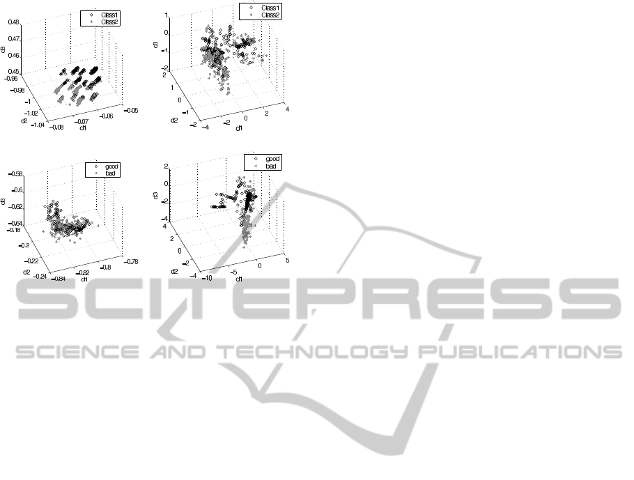
Figure 1: Projection into 3 dimensions of the australian and
ionosphere datasets (Bache and Lichman, 2013) using Au-
toencoders and Isomap. Representations (a) and (d) appear
to be more suitable for the classification tasks than the oth-
ers.
to the definition and are potentially usable for dimen-
sion reduction. An overview can be found in (Van der
Maaten et al., 2009) and (Ma and Fu, 2011). Ex-
amples of linear transforms are e.g. Principal Com-
ponent Analysis (PCA) or Linear Discriminant Anal-
ysis (LDA). Nonlinear techniques are e.g. Isomap,
Kernel-PCA or Local Linear Embedding (LLE). Par-
ticularly interesting are also Autoencoders, a special
form of neural networks that are also involved for the
training process in deep learning networks (Ngiam
et al., 2011). A list of manifold learning algorithms
with references can be found in the appendix.
3.3 Challenges for Classification
When manifold learning should be used for classifi-
cation applications there are three issues to consider.
First, many manifold learning algorithms have been
designed for artificial and noise-free data and fail
to produce reasonable models for real data (Van der
Maaten et al., 2009). The performance of a spe-
cific method heavily depends on the dataset. Fig-
ure 1 shows some example projections with Autoen-
coders (Hinton and Salakhutdinov, 2006) and Isomap
(Tenenbaum et al., 2000) on two different datasets.
The distributions of the projections and the usefulness
for the classification task are fairly different. This
makes it necessary to select a suitable algorithm for
each task.
Secondly, the out-of-sample extension is required
so that new instances can be embedded into the lower
dimensional feature space in a reasonable way. A di-
rect extension is available only for parametric meth-
ods (Van der Maaten et al., 2009), e.g. PCA and Au-
toencoders. For spectral methods, like LLE, Isomap
or Laplacian Eigenmaps, the Nystr¨om theorem (Ben-
gio et al., 2003) can be used for an extension. In the
following, the out-of-sample function of a manifold
learner refers to either the built-in extension or the
Nystr¨om extension method, depending on the avail-
ability.
And third, the intrinsic dimensionality d of the
manifold is not known. In real-world classification
applications, an optimal target dimensionality has to
be estimated and depends on the dataset, the mani-
fold learning algorithm and the classifier. Note that
this target dimensionality is not limited to 2 or 3 as it
is for visualization purposes.
4 HOLISTIC CLASSIFICATION
PIPELINE
In order to include feature selection, manifold learn-
ing techniques and classifiers into one holistic frame-
work a classification pipeline structure with 4 ele-
ments is proposed which is depicted in figure 1. Gen-
erally, the processing works like the pipes and filters
pattern (Buschmann et al., 1996) while the pipeline
has two modes: the training mode in which the train-
ing dataset T is needed and the classification mode in
which new samples can be classified. The idea is that
the dimensionalities
d
in
≥ d
FeatSel
≥ d
FeatTrans
≥ d
Label
= 1 (2)
of the feature vectors are typically decreasing while
they pass through the pipeline. The pipeline’s config-
uration θ describes a set of important hyperparame-
ters which have to be optimized for each learning task
(see section 5). The elements of the pipeline and their
contributions to θ are described in the following.
4.1 Feature Scaling Element
The first element of the pipeline is the feature scaling
element. Machine learning algorithms usually per-
form better when the numeric features have a normal-
ized value domain like e.g. [0,1] which is used in this
framework. In training mode, the value ranges of each
component of T are calculated. The minimum and
maximum value of the lth feature vector component
are denoted as minVal
l
and maxVal
l
, respectively. In
classification mode, each component of new vectors
RepresentationOptimizationwithFeatureSelectionandManifoldLearninginaHolisticClassificationFramework
37
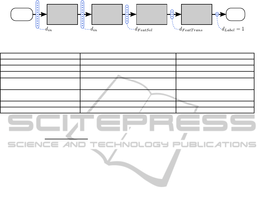
Feature
Transform
Element
Classifier
Element
Class
Label
Feature
Selection
Element
Input
Instance
Feature
Scaling
Element
Figure 2: Classifier concepts and corresponding hyperparameter grids and ranges.
Table 1: Classification pipeline structure to classify new instances when the configuration is known.
Classifiers discrete parameter grid continuous parameter ranges
Naive Bayes - -
C-SVM linear kernel C : {10
−2
,10
0
,10
2
} C : [10
−2
,10
4
]
C-SVM Gaussian kernel C : {10
−2
,10
0
,10
2
}, γ : {10
−4
,10
−1
,10
2
} C : [10
−2
,10
4
], γ : [10
−5
,10
2
]
k nearest neighbors (kNN) k : {1, 3,10}, metric: {Euclidean, Maha-
lan., Cityblock, Chebychev}
k : [1,20], metric: {Euclidean, Ma-
halan., Cityblock, Chebychev}
Multilayer Perceptron (MLP) hidden layers: {0,1, 2},
neurons per layer: {2,5,10}
hidden layers: [0,3],
neurons per layer: [1,10]
Extreme Learning Machine (ELM) neurons per layer: {10,20,50} neurons per layer: [1,100]
Random Forest number trees: {10,20,50} number trees: [1,50]
is transformed using
x
l
←
x
l
− minVal
l
maxVal
l
− minVal
l
. (3)
Note that this feature scaling doesn’t require any hy-
perparameters.
4.2 Feature Selection Element
The second element is the feature selection element
which contains the first dimension reduction. It re-
moves irrelevant and noisy feature dimensions that
could disturb any following algorithm. In training
mode, it selects a subset S
FeatSet
∈ P ({1, 2, ..., d
in
})\
/
0
of features. Feature selection is a difficult problem as
O(2
d
in
) possible combinations exist and it has a great
impact on the classification performance. Therefore,
it is included into the pipeline configuration θ. In
classification mode, the feature selection is performed
on vectors coming from the first element and the in-
put dimensionality is decreased from d
in
to d
FeatSel
=
|S
FeatSet
|.
4.3 Feature Transform Element
The third element is the feature transform element
which realizes the second dimension reduction with
manifold learning. The element contains a set of pos-
sible transformations S
FeatTrans
. Currently we use a
set of 16 functions provided by (Van der Maaten,
2014) which are listed in the appendix. We also in-
clude the identity function (no transform) in the set
as for some tasks, no feature transform might lead to
the best solution. The choice of a method f
FeatTrans
∈
S
FeatTrans
and the corresponding target dimensionality
d
FeatTrans
is included into the pipeline configuration θ.
The out-of-sample function of a feature transform
(see section 3.3) is crucial for the generalization per-
formance of the whole pipeline. Therefore, it has to
be included into the evaluation of the optimization
process and is described in section 5.1.
In classification mode, the chosen feature trans-
form model f
FeatTrans
is trained using the training
dataset T. New samples are embedded into the lower-
dimensional space using the out-of-sample function
and passed to the last pipeline element.
4.4 Classifier Element
The last element is the classifier element which uses a
classifier function f
Classifier
∈ S
Classifiers
. The frame-
work currently contains 7 “popular” multiclass ca-
pable classifier concepts which are listed in table
2. References to these concepts can be found e.g.
in (Bishop and Nasrabadi, 2006) and (Huang et al.,
2006). Each classifier can have an arbitrary number
of hyperparameters which are tuned during the opti-
mization phase (see section 5). Note that each clas-
sifier concept f
Classifier
has a different set of hyper-
parameters S
Params
( f
Classifier
) and both, the classifier
and its hyperparameters, are included into θ.
In training mode, the chosen classifier is trained
using the data processed by all previous pipeline ele-
ments while the labels stay the same as in the training
set T. In classification mode, the classifier classifies
the incoming vectors.
ICPRAM2015-InternationalConferenceonPatternRecognitionApplicationsandMethods
38
5 OPTIMIZATION OF THE
PIPELINE CONFIGURATION
The pipeline configuration finally contains all impor-
tant hyperparameters, namely
θ = (S
FeatSet
, f
FeatTrans
,d
FeatTrans
,
f
Classifier
,S
Params
( f
Classifier
)) (4)
which have to be optimized for each learning task.
First, a suitable evaluation metric has to be involved
to estimate the predictive performance of a pipeline
configuration. Secondly, the highly combinatorial
search problem to find the best configuration has to
be solved.
5.1 Optimization Target Function
The evaluation metric of a configuration θ plays a
central role as the generalization of the whole pipeline
needs to be evaluated. A common way to minimize
the risk of overfitting is k-fold cross-validation (Jain
et al., 2000). The feature transform element with its
out-of-sample function has a special role as the “intel-
ligence” is potentially moved from the classifier to the
feature transform: A highly nonlinear feature trans-
form might work best with a simple, e.g. linear clas-
sifier. However, simply transforming the whole train-
ing dataset T as a preprocessing step and performing
cross-validation afterwards never evaluates the gen-
eralization of the out-of-sample function on unseen
data. Therefore, it is necessary to incorporate the fea-
ture transform into the validation process.
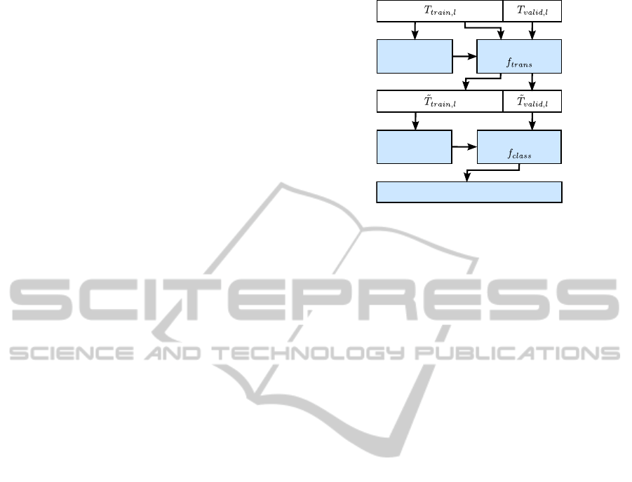
Each configuration θ is evaluated in the following
way (see figure 3). First, the feature selection is per-
formed. The training set T is separated into k = 5
cross-validation tuples with disjoint training and val-
idation datasets {(T
train,l
,T
valid,l
)}. For each cross-
validation round 1 ≤ l ≤ k the feature transform uses
T
train,l
to learn a model for feature transform. The
out-of-sample function of the derived model is used
to embed T
train,l
and T
valid,l
into the new feature space
to obtain (
˜
T
train,l
,
˜
T
valid,l
). Finally, the classifier is
trained with
˜
T
train,l
and the evaluation is done with
the predicted labels of
˜
T
valid,l
.
5.2 Evolution Strategies
Evolutionary optimization is well-suited to solve
high-dimensional and combinatorial optimization
problems. These algorithms imitate the biological
key strategy of evolving species over many genera-
tions. Especially evolution strategies (ES) are suitable
for the optimization of heterogeneous hyperparame-
ters (Beyer and Schwefel, 2002).
Learn feature
transform
Transformation
Train
classifier
Classifier
Evaluation
Figure 3: Evaluation of the lth cross-validation set to es-
timate the generalization of the feature transform and the
classifier at the same time.
The basic idea is to code the classification pipeline
configuration θ (see equation 4) into a suitable ge-
netic representation for the evolutionary operators in
ES strategies, namely random generation of individ-
uals, selection, recombination and mutation. In ES
parameters can conveniently be coded directly as real
or integer number search space R
N
and Z
N
with cor-
responding value ranges. The mutation operator for
these types is defined as an additive Gaussian noise
with covariance matrix Σ. Additionally, a bit string
search space B
N
(binary mask) as well as a discrete
set search space W to model categorical parameters
can be defined.
The parameters for the ES strategies can be coded
in the (µ/ρ + λ) notation. The number of individuals
that survive in each generation is denoted as µ. In each
generation λ children from ρ parents are derived. The
evaluation metric based on cross-validation described
in the previous section is used to determine the fit-
ness of the individuals. One big advantage of ES al-
gorithms is that the calculation of the fitness values of
a population can easily be parallelized. These fitness
values are needed for selection and recombination so
that the fittest individuals survive and evolve. Two
different optimization strategies are presented:
5.3 Evolutionary Grid Search
The first algorithm is an evolutionary grid search
(EGS) that codes the feature subset, feature transform,
target dimensionality d
FeatTrans
and classifier into the
chromosome. The feature subset is coded as binary
mask B
d
in
which is similar to e.g. (Huang and Wang,
2006). The feature transform and classifier concept
are both coded as the set genotype W. For the tar-
get dimensionality a factor α ∈ [0,1] is coded as R
1
genotype. It determines the fraction of the number
of dimensions delivered by the feature selection that
RepresentationOptimizationwithFeatureSelectionandManifoldLearninginaHolisticClassificationFramework
39
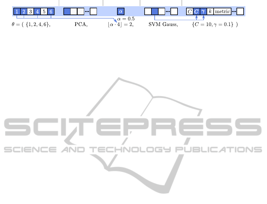
Feature transform Dim. fraction
Feature subset
Classifier hyperparameters
Classifier
Figure 4: Exemplary coding schema of a pipeline configuration θ for the CE strategy. The EGS coding schema is similar, but
no classifier hyperparameters are appended.
should be used as target dimensionality
d
FeatTrans
= ⌊α · d
FeatSel
⌋ , d
FeatTrans
≥ 1. (5)
The corresponding hyperparameters of the se-
lected classifier are optimized using grid search with
the grids from the middle column in table 2. An ini-
tial population of 250 random individuals is gener-
ated to start the ES with parameters µ = 50, ρ = 2
and λ = 100. A mutation probability of p
Mut
= 0.3 is
used for both feature subset bit flips and the discrete
set type W to pick a random item. The algorithm ter-
minates when the improvement of the best fitness is
less than ε = 10
−4
after at least 3 generations.
5.4 Complete Evolutionary
Optimization
The second algorithm is the complete evolutionary
optimization (CE) which is based on the EGS strat-
egy but no grid search of the classifiers’ hyperparam-
eters has to be made as they are included into the
genomes. The problem with optimizing all parame-
ters of all classifiers in a single evolutionary way is
that each classifier concept has its own set of inde-
pendent hyperparameters. To solve this, all hyperpa-
rameters with their corresponding types are appended
to the genome consecutively. The classifier selection
acts like a switch which “activates” the correspond-
ing hyperparameters while those from other classi-
fiers remain unused. However, all hyperparameters
are evolved with the evolutionary operators in par-
allel. Figure 4 illustrates this coding and activation
scheme. The advantage of this approach is that pa-
rameters ranges can be continuous and allow a much
finer adaptation to the classification task. Further-
more, no exhaustive grid search is needed. The right
column in table 2 shows the hyperparameter ranges
for the CE strategy that are used in the framework.
As the evolutionary search space is larger now,
some parameters have to be changed compared to
EGS. The initial population is changed to 500 individ-
uals and the number of generated children to λ = 200.
For mutation of integer and floating point parameters
a variance of Σ = 2 is used. In order to handle expo-
nentially ranged real valued hyperparameters of the
classifiers (e.g. C and γ for the SVM) in the same
framework, the exponent log
10
(x) is used for geno-
type coding.
5.5 Multi-pipeline Classifier
All presented optimization methods lead to a result
list of N
Res
configurations R = {(θ
j
,q
j
)}, 1 ≤ j ≤
N
Res
with a corresponding fitness q
j
. The configu-
rations can be sorted by their fitness q
j
and, at first
glance, the configuration with the highest fitness is
the most interesting result. However, this solution
could be randomly picked and therefore quite “un-
usual” and also potentially overfitted to the training
set, even though cross-validation is used.
The distribution of the top-n configurations can be
used to generate a multi-pipeline classifier. Multi-
classifier systems have the potential to improve the
generalization capabilities compared to a single clas-
sifier when the diversity of the different models is
large enough (Ranawana and Palade, 2006). A multi-
pipeline classifier is defined such that the top-n con-
figurations are used to set up n pipelines with the cor-
responding configuration θ
j
. In classification mode,
all pipelines are classifying the input vector parallelly
and finally, the most frequent label of all predictions
is chosen (majority voting).
6 EXPERIMENTS
For the evaluation of the presented framework 10
classification problems from the UCI database (Bache
and Lichman, 2013) have been used with different di-
mensionalities, number of samples and classes (see
table 2). In order to test the generalization capabil-
ities the instances of all datasets have been divided
randomly into 50% train and 50% test sets. The two
optimization strategies EGS and CE are evaluated and
compared to a baseline classifier which is an SVM
with a Gaussian kernel, using the full feature set, no
feature transform and optimally grid-based tuned hy-
perparameters.
The proposed evolutionary algorithms use random
components which may lead to non-reproducible re-
sults and local maxima. In order to overcome this
problem in the evaluations, all experiments have been
repeated 5 times. In the following sections and tables
ICPRAM2015-InternationalConferenceonPatternRecognitionApplicationsandMethods
40
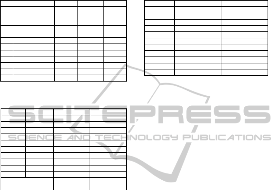
Table 2: Dataset information. Note that the datasets are
ordered by their dimensionality.
Dataset dim. samples classes
1 iris 4 150 3
2 pima-indians-
diabetes
8 768 2
3 breast-cancer-
wisconsin
9 683 2
4 contraceptive 9 1473 3
5 glass 9 214 6
6 statlogheart 13 270 2
7 australian 14 690 2
8 vehicle 18 846 4
9 ionosphere 34 351 2
10 sonar 60 208 2
Table 3: Average optimization cross-validation accuracy
and average improvements to baseline SVM of the differ-
ent strategies.
Dataset Baseline EGS CE
1 94.67 98.67 ± 0.00 98.67 ± 0.00
2 77.34 81.10 ± 0.57 80.89 ± 0.63
3 97.07 98.24 ± 0.00 98.30 ± 0.13
4 52.84 55.12 ± 0.35 54.34 ± 0.89
5 60.56 80.02 ± 1.56 79.94 ± 2.62
6 84.44 88.00 ± 0.62 87.41 ± 0.52
7 86.14 87.93 ± 0.24 88.21 ± 0.65
8 79.46 80.51 ± 0.79 82.68 ± 1.07
9 91.49 95.60 ± 0.74 95.95 ± 0.26
10 84.76 87.62 ± 0.95 87.62 ± 1.35
Average improve-
ment to baseline
+4.40 ± 5.41 +4.52 ± 5.32
the averages and – if enough space is available – the
standard deviations are presented and discussed. Cur-
rently, the framework is implemented in Matlab using
the Parallel Computing Toolbox and is run on an Intel
Xeon workstation with 6 × 2.5Ghz.
6.1 Evaluation of Optimization
Strategies
First, the optimization process on the training dataset
is evaluated. The best cross-validation accuracies af-
ter the optimization with the EGS and CE strategy
can be found in table 3. Both strategies achieve sig-
nificantly higher cross-validation accuracies than the
SVM baseline for all datasets. The differences are
small, but the CE strategy performs slightly better
for 6 of 10 datasets with an average accuracy gain of
+4.52% compared to the SVM baseline. This shows
that the proposed pipeline structure and optimization
allows a high adaptation to the learning task compared
to a standard SVM.
The optimization times per dataset are listed in ta-
ble 4. The optimization times vary from a few min-
Table 4: Average optimization times for each dataset and
the two strategies in minutes.
Dataset EGS CE
1 6.42 ± 0.47 6.65 ± 0.95
2 85.53 ± 38.63 115.31 ± 35.76
3 25.60 ± 5.85 38.94 ± 2.52
4 129.88 ± 17.79 229.18 ± 44.99
5 13.69 ± 2.07 20.51 ± 3.49
6 23.79 ± 5.85 37.76 ± 9.34
7 58.03 ± 11.34 82.33 ± 23.59
8 75.93 ± 12.35 137.55 ± 23.30
9 12.58 ± 2.34 17.48 ± 2.21
10 8.67 ± 1.23 11.56 ± 1.33
Average 44.01 ± 41.67 69.73 ± 72.07
utes to several hours. On average the optimization
time is around 44 minutes for the EGS and around
70 minutes for the CE strategy. This is an interest-
ing observation as the CE strategy does not need ex-
haustive grid search like EGS. On the other hand,
the search space for the continuous hyperparameter
ranges is much larger and thus more time is needed
for the evolution of good parameter values. Inter-
estingly, the optimization time is not correlated with
the dataset dimensionality, but depends on the feature
transforms and classifiers that are used as the training
time of these is fairly different.
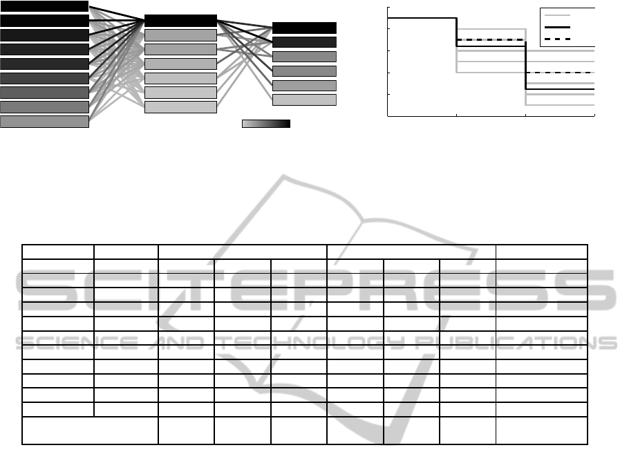
The distribution of the best configurations in R
can be analyzed to get insight into the classification
problem and its solutions. Figure 5 (a) visualizes an
exemplary result of the top-50 configurations of the
CE strategy for the breast-cancer-wisconsin dataset as
a graph. It shows the distribution of frequencies of
features, feature transforms, classifiers and the con-
nections between them with a different shading of
boxes and edges. The components and connections
which are included in the overall best configuration
are marked with an asterisk (*).
The feature distribution is especially useful to
measure the importance of single features. The large
variety of feature transforms in the best configurations
indicates that the feature distribution contains a lower
dimensional manifold which can be used for a better
feature representation. Additionally, two rather sim-
ple classifiers, namely the naive Bayes and the kNN
classifier, appear as the most frequently chosen classi-
fiers. This shows the benefit of the feature transforms
so that no complex classifier model is needed.
Figure 5 (b) shows a exemplary visualization of
the distribution of dimensionalities which is helpful to
analyze the intrinsic dimensionality of a classification
problem. The aforementioned top-50 configurations
are analyzed with respect to the dimensionalities of
the feature selection (d
FeatSel
) and the feature trans-
form element (d
FeatTrans
). It can be seen that around 6
RepresentationOptimizationwithFeatureSelectionandManifoldLearninginaHolisticClassificationFramework
41
BareNuclei*
ClumpThickness*
UniformityCellShape*
MarginalAdhesion*
BlandChromatin*
Mitoses*
SingleEpithelialCellSize
UniformityCellSize*
NormalNucleoli
Factor Analysis
Kernel−PCA Poly*
LDA
Auto Encoder
LPP
PCA
Kernel−PCA Gauss
Naive Bayes*
kNN
SVM linear
ELM
SVM Gauss
Random Forest
Frequency
(a) Top configuration graph.
Input Feature Selection Feature Transform Classifier
0
2
4
6
8
10
all
mean
best
(b) Dimensionality distribution.
Figure 5: Graphical analyses of the top-50 configuration distribution for the breast-cancer-wisconsin dataset using the CE
strategy. Figure (a) shows the distribution of features, feature transforms and classifiers as a graph. Figure (b) shows the
distribution of the selected dimensionalities for the different pipeline elements.
Table 5: Average accuracy results on test datasets in % depending on different optimization strategies and a different number
of top-n multi-pipeline configurations compared to baseline SVM and Auto-WEKA with a time budget of 24 hours.
Dataset Baseline EGS CE Auto-WEKA
Top-1 Top-10 Top-20 Top-1 Top-10 Top-20
1 100.00 94.67 94.40 94.93 96.00 96.80 97.60 92.27
2 76.82 74.79 74.95 75.31 75.83 75.47 75.42 75.83
3 95.89 96.89 96.66 96.66 95.89 96.48 96.36 96.72
4 53.20 55.59 57.55 57.80 55.84 56.76 57.47 57.17
5 66.67 66.67 70.48 71.05 72.38 72.95 74.10 74.86
6 83.70 82.96 83.70 83.26 82.07 83.26 82.52 83.70
7 84.88 86.16 85.64 85.87 85.41 85.29 85.17 85.29
8 80.81 77.87 79.72 79.34 80.43 82.80 82.89 81.18
9 94.29 94.40 95.89 96.57 93.37 96.57 96.69 96.11
10 79.61 82.33 85.24 85.44 81.36 87.57 87.77 85.63
Average difference
to baseline
-0.35
± 2.50
+0.83
± 3.30
+1.04
± 3.34
+0.27
± 2.64
+1.81
± 3.41
+2.01
± 3.64
+1.29 ± 4.32
of the 9 input dimensions are relevant for the feature
selection while the remaining data appears to be on a
2 or 3 dimensional manifold. This consecutivedimen-
sion reduction is very typical for most of the datasets
that have been investigated.
6.2 Generalization on Test Datasets
The results of the proposed framework on the test
datasets can be found in table 5. First, the results of
the best single configurations (top-1 columns) of the
EGS and CE strategies are considered. The average
differences compared to the baseline show that the
configurations derived with the CE strategy slightly
outperform the ones from the EGS strategy. How-
ever, the difference is marginal and in many cases,
even the baseline SVM performs better. The high ac-
curacy gains during training are not reached for the
test datasets which indicates that pipelines tend to be
overfitted even though cross-validation is used.
The multi-pipeline classifiers (see section 5.5)
with the top-10 and top-20 pipelines show a much
better generalization on the test data than the top-1
pipeline alone. Especially configurations of the CE
strategy profit from the multi-pipeline classifier. It
can be observed in many cases that the performance
increases when more pipelines are used. The high-
est average difference compared to the baseline is
achieved with the fusion of the top-20 pipelines of
the CE strategy with +2.01% . However, the specific
benefit of a certain strategy and a certain number of
pipelines depends on the dataset.
Furthermore, the results have been compared to
the Auto-WEKA framework (see section 2) with
a time budget of 24 hours and 5 repetitions for
each dataset. The average accuracies beat the top-
1 pipelines of the EGS and CE strategy in 6 of 10
cases which shows that the classifier systems of the
Auto-WEKA framework are less overfitted. When
the multi-pipeline classifiers are compared, the solu-
tions of Auto-WEKA only perform better or equal in
2 cases.
7 CONCLUSIONS
In this work, a holistic classification pipeline frame-
work with feature selection, multiple manifold learn-
ing techniques, multiple classifiers and hyperparam-
ICPRAM2015-InternationalConferenceonPatternRecognitionApplicationsandMethods
42

eter optimization has been presented. The portfolio
of manifold learners and classifiers is exchangeable
so that new algorithms can be plugged in and com-
pared quickly. Two evolutionary optimization strate-
gies have been presented that solve the highly combi-
natorial optimization process to find the best pipeline
configuration and data representation. An adapted
variant of cross-validation is used that estimates the
generalization performance of the feature transform
and classifier. The framework is easy to use as the
user only needs to provide a labeled training dataset
and obtains a solution within a range of several min-
utes to a few hours. Additionally, analyses of the best
configurations help to reveal information about latent
properties of the feature data, e.g. the importance of
features, manifold-like distributions and intrinsic di-
mensionalities.
The evaluation of the framework shows that the
cross-validation accuracies during training increase
significantly compared to the baseline SVM. How-
ever, the best configurations tend to be overfitted
to the training dataset even though cross-validation
with incorporation of the feature transform is used.
Generally, the fusion of multiple pipelines shows a
much better performance and outperforms the base-
line as well as the results obtained by the Auto-
WEKA framework on most of the datasets. Alto-
gether, the CE optimization strategy performs best on
average.
The generalization performance of the proposed
framework needs to be investigated further to over-
come evident overfitting effects. A central question is
which pipeline element – feature selection or feature
transform – has the biggest effect on the generaliza-
tion. The concept of multi-pipeline classifiers offers
a better performance, but comes along with higher
computational costs. Future work will analyze the in-
terplay of the number of pipelines and the diversity of
the configuration set for the multi-pipeline classifier.
Additionally, many manifold learning techniques also
have hyperparameters that should also be optimized
automatically. Furthermore, the framework will be
tested for classification problems with higher dimen-
sional features such as raw pixel data for image-based
object recognition to test the scalability regarding the
computational cost. Finally, an open-source publica-
tion of the software framework is planned.
ACKNOWLEDGEMENTS
This work was funded by the European Com-
mission within the Ziel2.NRW programme
“NanoMikro+Werkstoffe.NRW”.
REFERENCES
˚
Aberg, M. and Wessberg, J. (2007). Evolutionary optimiza-
tion of classifiers and features for single trial eeg dis-
crimination. Biomedical engineering online, 6(1):32.
Bache, K. and Lichman, M. (2013). UCI machine learning
repository.
http://archive.ics.uci.edu/ml/
.
Belkin, M. and Niyogi, P. (2001). Laplacian eigenmaps and
spectral techniques for embedding and clustering. In
Advances in Neural Information Processing Systems
(NIPS), volume 14, pages 585–591.
Bengio, Y. (2000). Gradient-based optimization of hyper-
parameters. Neural computation, 12(8):1889–1900.
Bengio, Y., Courville, A., and Vincent, P. (2013). Represen-
tation learning: A review and new perspectives. Pat-
tern Analysis and Machine Intelligence, IEEE Trans-
actions on, 35(8):1798–1828.
Bengio, Y., Paiement, J.-f., Vincent, P., Delalleau, O., Roux,
N. L., and Ouimet, M. (2003). Out-of-sample exten-
sions for lle, isomap, mds, eigenmaps, and spectral
clustering. In Advances in Neural Information Pro-
cessing Systems, page None.
Bergstra, J., Bardenet, R., Bengio, Y., K´egl, B., et al.
(2011). Algorithms for hyper-parameter optimiza-
tion. In 25th Annual Conference on Neural Informa-
tion Processing Systems (NIPS 2011).
Bergstra, J. and Bengio, Y. (2012). Random search for
hyper-parameter optimization. J. Mach. Learn. Res.,
13(1):281–305.
Beyer, H.-G. and Schwefel, H.-P. (2002). Evolution strate-
gies - a comprehensive introduction. Natural Comput-
ing, 1(1):3–52.
Bishop, C. M. and Nasrabadi, N. M. (2006). Pattern recog-
nition and machine learning, volume 1. Springer New
York.
Brand, M. (2002). Charting a manifold. In Advances in neu-
ral information processing systems, pages 961–968.
MIT Press.
B¨urger, F., Buck, C., Pauli, J., and Luther, W. (2014).
Image-based object classification of defects in steel
using data-driven machine learning optimization. In
Braz, J. and Battiato, S., editors, Proceedings of Inter-
national Conference on Computer Vision Theory and
Applications (VISAPP), pages 143–152.
Buschmann, F., Meunier, R., Rohnert, H., Sommerlad, P.,
Stal, M., and Stal, M. (1996). Pattern-Oriented Soft-
ware Architecture Volume 1: A System of Patterns.
Wiley.
Donoho, D. L. and Grimes, C. (2003). Hessian eigen-
maps: Locally linear embedding techniques for high-
dimensional data. Proceedings of the National
Academy of Sciences, 100(10):5591–5596.
Fisher, R. A. (1936). The use of multiple measurements in
taxonomic problems. Annals of Eugenics, 7(2):179–
188.
Fukumizu, K., Bach, F. R., and Jordan, M. I. (2004). Di-
mensionality reduction for supervised learning with
reproducing kernel hilbert spaces. J. Mach. Learn.
Res., 5:73–99.
RepresentationOptimizationwithFeatureSelectionandManifoldLearninginaHolisticClassificationFramework
43

Globerson, A. and Roweis, S. T. (2005). Metric learning by
collapsing classes. In Advances in neural information
processing systems, pages 451–458.
Goldberger, J., Roweis, S., Hinton, G., and Salakhutdinov,
R. (2004). Neighbourhood components analysis. In
Advances in Neural Information Processing Systems
17.
He, X., Cai, D., Yan, S., and Zhang, H.-J. (2005). Neigh-
borhood preserving embedding. In Computer Vision
(ICCV), 10th IEEE International Conference on, vol-
ume 2, pages 1208–1213.
Hinton, G. E. and Salakhutdinov, R. R. (2006). Reducing
the dimensionality of data with neural networks. Sci-
ence, 313(5786):504–507.
Huang, C.-L. and Wang, C.-J. (2006). A GA-based fea-
ture selection and parameters optimizationfor support
vector machines. Expert Systems with Applications,
31(2):231 – 240.
Huang, G.-B., Zhu, Q.-Y., and Siew, C.-K. (2006). Extreme
learning machine: theory and applications. Neuro-
computing, 70(1):489–501.
Huang, H.-L. and Chang, F.-L. (2007). Esvm: Evolution-
ary support vector machine for automatic feature se-
lection and classification of microarray data. Biosys-
tems, 90(2):516 – 528.
Jain, A. K., Duin, R. P. W., and Mao, J. (2000). Statistical
pattern recognition: a review. Pattern Analysis and
Machine Intelligence, IEEE Transactions on, 22(1):4–
37.
Kim, H., Howland, P., and Park, H. (2005). Dimension re-
duction in text classification with support vector ma-
chines. In Journal of Machine Learning Research,
pages 37–53.
Ma, Y. and Fu, Y. (2011). Manifold Learning Theory and
Applications. CRC Press.
Ngiam, J., Coates, A., Lahiri, A., Prochnow, B., Le, Q. V.,
and Ng, A. Y. (2011). On optimization methods for
deep learning. In Proceedings of the 28th Interna-
tional Conference on Machine Learning (ICML-11),
pages 265–272.
Niyogi, X. (2004). Locality preserving projections. In Neu-
ral information processing systems, volume 16, page
153.
Pearson, K. (1901). On lines and planes of closest fit to
systems of points in space. The London, Edinburgh,
and Dublin Philosophical Magazine and Journal of
Science, 2(11):559–572.
Ranawana, R. and Palade, V. (2006). Multi-classifier sys-
tems: Review and a roadmap for developers. Interna-
tional Journal of Hybrid Intelligent Systems, 3(1):35–
61.
Sch¨olkopf, B., Smola, A., and M¨uller, K.-R. (1998). Non-
linear component analysis as a kernel eigenvalue prob-
lem. Neural computation, 10(5):1299–1319.
Spearman, C. (1904). “general intelligence”, objectively
determined and measured. The American Journal of
Psychology, 15(2):201–292.
Tenenbaum, J. B., De Silva, V., and Langford, J. C. (2000).
A global geometric framework for nonlinear dimen-
sionality reduction. Science, 290(5500):2319–2323.
Thornton, C., Hutter, F., Hoos, H. H., and Leyton-Brown,
K. (2013). Auto-WEKA: Combined selection and
hyperparameter optimization of classification algo-
rithms. In Proc. of KDD-2013, pages 847–855.
Van der Maaten, L. (2014). Matlab Toolbox for Dimension-
ality Reduction.
http://homepage.tudelft.nl/
19j49/Matlab_Toolbox_for_Dimensionality_
Reduction.html
.
Van der Maaten, L., Postma, E., and Van Den Herik, H.
(2009). Dimensionality reduction: A comparative re-
view. Journal of Machine Learning Research, 10:1–
41.
Weinberger, K. Q. and Saul, L. K. (2009). Distance metric
learning for large margin nearest neighbor classifica-
tion. Journal of Machine Learning Research, 10:207–
244.
Wolpert, D. H. (1996). The lack of a priori distinctions
between learning algorithms. Neural computation,
8(7):1341–1390.
Zhang, T., Yang, J., Zhao, D., and Ge, X. (2007). Linear
local tangent space alignment and application to face
recognition. Neurocomputing, 70(7):1547–1553.
APPENDIX
List of manifold learning methods that are used in the
framework, including references and abbreviations:
Principal Component Analysis (PCA) (Pearson,
1901), Kernel-PCA with polynomial and Gaussian
kernel (Sch¨olkopf et al., 1998), Denoising Autoen-
coder (Hinton and Salakhutdinov, 2006), Local Lin-
ear Embedding (LLE) (Donoho and Grimes, 2003),
Isomap (Tenenbaum et al., 2000), Manifold Chart-
ing (Brand, 2002), Laplacian Eigenmaps (Belkin and
Niyogi, 2001), Linear Local Tangent Space Align-
ment algorithm (LLTSA) (Zhang et al., 2007), Lo-
cality Preserving Projection (LPP) (Niyogi, 2004),
Neighborhood Preserving Embedding (NPE) (He
et al., 2005), Factor Analysis (Spearman, 1904),
Linear Discriminant Analysis (LDA) (Fisher, 1936),
Maximally Collapsing Metric Learning (MCML)
(Globerson and Roweis, 2005), Neighborhood Com-
ponents Analysis (NCA) (Goldberger et al., 2004),
Large-Margin Nearest Neighbor (LMNN) (Wein-
berger and Saul, 2009).
ICPRAM2015-InternationalConferenceonPatternRecognitionApplicationsandMethods
44
