
Joint Under and Over Water Calibration
of a Swimmer Tracking System
Sebastian Haner, Linus Sv
¨
arm, Erik Ask and Anders Heyden
Centre for Mathematical Sciences, Lund University, Lund, Sweden
Keywords:
Underwater Imaging, Camera Calibration, Refraction, Stitching.
Abstract:
This paper describes a multi-camera system designed for capture and tracking of swimmers both above and
below the surface of a pool. To be able to measure the swimmer’s position, the cameras need to be accurately
calibrated. Images captured below the surface provide a number of challenges, mainly due to refraction
and reflection effects at optical media boundaries. We present practical methods for intrinsic and extrinsic
calibration of two sets of cameras, optically separated by the water surface, and for stitching panoramas
allowing synthetic panning shots of the swimmer.
1 INTRODUCTION
In competitive swimming, being able to measure and
analyze a swimmer’s movements during training can
be very useful in identifying weaknesses and for
tracking progress. In this paper we describe parts of
a real-time computer vision system designed for this
purpose, with focus on the calibration of the camera
rig and the problems of underwater imaging arising
from refraction effects.
First we consider the problem of calibrating a
combined over– and underwater camera setup. Cal-
ibration is necessary to be able to compute the swim-
mer’s position from image projections, and to gener-
ate synthetic panning views following the swimmer
using stationary cameras. In Section 3, we describe
the process of intrinsic and extrinsic calibration, and
how we deal with the problems arising from refrac-
tion and reflection at optical media boundaries.
The second problem we consider in this paper re-
gards generating visually pleasing images from the
cameras. To accomplish this, all geometric distortions
must be neutralized along with lens vignetting, chro-
matic aberration and exposure variations. In Section
4, we present practical methods for achieving these
goals, and for stitching together images from the sta-
tionary cameras allowing synthetic panning shots of
the swimmer.
To illustrate the effectiveness of our approach we
conclude the paper with full-length stitched over– and
underwater panoramas of the pool along with exam-
ple output from the complete vision system.
1.1 Related Work
The literature on camera calibration is vast and spans
many decades, but the calibration of cameras un-
der refraction has received little attention until re-
cently. (Agrawal et al., 2012) present a method for
determining camera pose and refractive plane param-
eters from a single image of a known calibration ob-
ject using eight point correspondences. (Chang and
Chen, 2011) solves the relative and absolute pose
problems of cameras observing structure through a
common horizontal flat refractive surface, given that
the gravity vector is known, while (Jordt-Sedlazeck
and Koch, 2013) rely on iterative optimization for
determining relative and absolute pose when the re-
fractive planes are known relative to the cameras.
(Kang et al., 2012) solve relative and absolute pose
optimally under the L
∞
-norm given known rotations.
However, in the application considered here, relative
poses of the cameras and refractive plane parame-
ters are known to a sufficient degree so that only
the absolute pose of a calibration object needs to be
computed before non-linear iterative optimization is
applied. In (Jordt-Sedlazeck and Koch, 2013) effi-
cient refractive bundle adjustment is performed using
the Gauss-Helmert model; in contrast, our method of
computing the forward projection through refractive
media allows bundle adjustment using standard non-
linear least-squares solvers which typically do not im-
plement equality constraints.
142
Haner S., Svärm L., Ask E. and Heyden A..
Joint Under and Over Water Calibration of a Swimmer Tracking System.
DOI: 10.5220/0005183701420149
In Proceedings of the International Conference on Pattern Recognition Applications and Methods (ICPRAM-2015), pages 142-149
ISBN: 978-989-758-077-2
Copyright
c
2015 SCITEPRESS (Science and Technology Publications, Lda.)
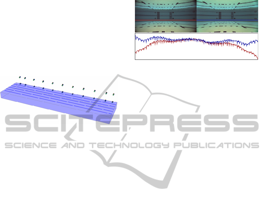
2 CAMERA SETUP
The system consists of two rows of cameras mounted
along the long edge of a 50 m swimming pool; one
row looking down at the surface from above, and one
row below the water line observing the pool through
glass windows (see Figure 1). The cameras are ori-
ented to observe one of the lanes in the pool. All
cameras are synchronized so that matches of mov-
ing calibration markers between cameras are known
to correspond to the same spatial location.
Figure 1: The system setup with two rows of cameras along
the pool observing the middle lane.
3 CALIBRATION
The aim of calibration is to determine the intrinsic
and extrinsic parameters of all the cameras in a joint
coordinate system. The system at hand presents two
major difficulties: the underwater cameras experience
refraction effects at the air–glass and glass–water in-
terfaces, and total internal reflection at the water sur-
face means no objects above the surface are visible
to the underwater cameras. Likewise, unpredictable
refraction effects due to surface waves means obser-
vations of underwater objects from above the pool are
unreliable.
The calibration process consists of the following
steps:
1. Intrinsic in-air calibration of all cameras
2. Capture calibration object
3. Detect calibration markers
4. Initialize calibration object pose and camera ex-
trinsic parameters
5. Refine parameters using bundle adjustment.
Below, we describe these in more detail.
3.1 Intrinsic Calibration
All cameras are calibrated in air, i.e. without the re-
fractive interface, recovering focal length, principal
point and lens distortion parameters prior to full sys-
tem calibration. We use the standard method (Zhang,
Figure 2: Devignetting result. On the left the original im-
age, on the right the devignetted and below the intensity
profiles of the indicated lines. The vignetting effect is se-
vere near the corners of the image and cannot be corrected
with the adopted model. However, these parts of the image
are not used in the panorama generation due to the horizon-
tal overlap between cameras.
1999) and the distortion model of (Heikkila and Sil-
ven, 1997). The wide-angle lenses used also exhibit a
significant degree of vignetting which must be com-
pensated for to produce seamless stitching of the im-
ages. We model each color channel of the vignetted
image as I
vig
(r,θ) = I(r,θ)(1 + c
1
r
2
+ c
2
r
4
+ c
3
r
6
)
where the origin is taken to be the recovered princi-
pal point. The parameters c
i
can be estimated inde-
pendently for each channel using linear least-squares
fitting to images taken of evenly lit single-color flat
surfaces. For the underwater cameras, we use images
of the opposite pool wall for this purpose, taken af-
ter the cameras have been mounted. This ensures the
vignetting effect produced by Fresnel reflection at the
glass interfaces is also accounted for, although it is
quite weak. Figure 2 shows a result of the method.
3.2 The Calibration Object
As mentioned above, total internal reflection and sur-
face waves means no single point can be observed
simultaneously by both an underwater and a wall-
mounted camera. The solution is to use a semi-
submersed known rigid calibration object, different
parts of which can be observed simultaneously by the
two sets of cameras. The object was chosen as a ver-
tical straight rod with easily recognizable markings at
known intervals; we used eight bright-yellow balls,
four mounted below and four above a polystyrene
foam flotation device. A more elaborate rig with two–
or three-dimensional structure would give additional
calibration constraints, but also be more unwieldy and
difficult to construct and use. The floating rig is towed
around the pool while capturing images making sure
to cover each camera’s field of view.
JointUnderandOverWaterCalibrationofaSwimmerTrackingSystem
143
Figure 3: The cameras mounted below the waterline only
see the bottom half of the calibration object, and the wall-
mounted cameras only the top half.
3.3 Marker Detection
The marker detection and localization is performed
in three steps. First all pixels are classified based on
color content using a support vector machine (SVM)
on a transformed color space, then the SVM response
map is thresholded and connected components are
identified. The obtained regions are then filtered with
respect to shape to obtain the final potential marker
locations used for solving the pose problem (see Sec-
tion 3.4).
3.3.1 SVM and Color Transform
The markers have uniform and distinct color. How-
ever, due to light absorption in water, the color in the
underwater cameras varies with distance. The avail-
able fluorescent lighting above the pool has a fairly
narrow spectrum which also makes color differentia-
tion more difficult. In addition, specularities and re-
flections in the water surface may also appear yellow.
For these reasons a linear SVM classifier based only
on RGB channels proved insufficient for segmenting
the markers. To mitigate the issues of varying light
conditions, and improve the detection of yellow, the
images are converted to the CMYK color space with
the non-linear transformation
K = min(1 −R,1 − G,1 − B)
C =
1 − R − K
1 − K
M =
1 − G − K
1 − K
Y =
1 − B − K
1 − K
.
(1)
To further augment the input data to the SVM, all sec-
ond order combinations of the chromatic components
are added to the feature vector. For each pixel p
k
the
Figure 4: Example of SVM performance. The calibration
tool and the SVM response. The SVM is trained on a dif-
ferent sample image.
feature v
k
is taken as
v
k
=
C, M, Y, C
2
, M
2
, Y
2
, CM, CY, MY, K
T
k
,
with [C, M, Y, K]
k
the color information at the pixel
location.
Separate classifiers are constructed for over and
underwater cameras using the standard linear soft
margin SVM formulation, solving
min
W,b,ζ
1
2
W
T
W +C
∑
k
ζ
k
s.t. t
k
W
T
v
k
+ b
− 1 ≥ 1 − ζ
k
, k = 1,...,N
ζ
k
≥ 0, k = 1,...,N ,
where W , b are the sought SVM parameters, ζ an
allowance of points being placed on the wrong side
of the hyperplane, and t
k
a {−1,1} indicator. Posi-
tive and negative samples are extracted from a single
representative image for each of the classifiers. The
penalty C is selected to be fairly large while still giv-
ing feasible solutions.
A representative example of the detection using
the trained SVM is shown in Figure 4.
3.3.2 Region Properties
As the markers are spherical the sought regions
should be conics. A reasonable simplification is to
search for approximately circular regions. A simple
confidence measure of how circular a region is was
devised as the following:
1. Discard all regions whose area is smaller than a
disc of radius 5 pixels or larger than a disc of ra-
dius 50.
ICPRAM2015-InternationalConferenceonPatternRecognitionApplicationsandMethods
144
2. Estimate two radii (r
min
, r
max
) based on the re-
gions’ second order moments, i.e. do ellipse fit-
ting.
3. Create two circular regions around the centre with
the sizes r
min
and 3r
min
.
4. Score based on the ratio of region inside the inner
circle to region in the larger circle.
Regions are then culled based on relative response
where regions whose confidence is below a ratio of
20% of the maximum confidence are discarded. The
midpoints of the remaining regions are used as candi-
dates for the markers when solving for the calibration
stick pose.
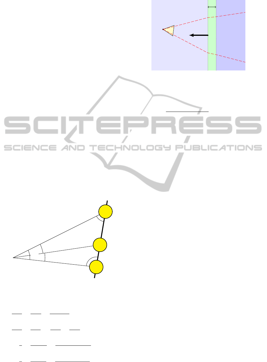
3.4 Solving for the Stick Pose
We model the stick as points on a line. The pose
of the stick relative to a perspective camera can be
uniquely determined (up to rotation around its own
axis) from the projection of three markers in a sin-
gle image, given their absolute positions on the stick.
Unlike the general 3-point pose problem, where the
points are not collinear, this can be solved easily in
closed form using simple trigonometry. Consider Fig-
ure 5, where C represents the known camera center
and D
1,2
the known distances between the markers. If
we can compute two of the depths x, y or z, the pose
relative to the camera can be inferred. From the law
C
M
1
M
2
M
3
γ
β
α
ε
δ
x
y
z
D
1
D
2
Figure 5: Three markers on the calibration rod viewed by a
camera.
of sines we have
sinε
y
=
sinδ
x
=
sinα
D
1
+ D
2
,
sinε
z
=
sinγ
D
1
,
sinδ
z
=
sinβ
D
2
⇒
z
x
=
sinδ/x
sinδ/z
=
D
2
sinα
(D
1
+ D
2
)sinβ
≡ K
x
z
y
=
sinε/y
sinε/z
=
D
1
sinα
(D
1
+ D
2
)sinγ
≡ K
y
.
(2)
d
~n
W
n
1
n
2
n
3
C
Figure 6: Each underwater camera C views the pool through
a glass pane of thickness d mounted at W and with normal
vector~n.
From the law of cosines, D
2
1
= x
2
+ z
2
−
2xz cosγ. Substituting z = xK
x
, solve for
x = D
1
/
p
K
2
x
− 2K
x
cosγ + 1 and y = xK
x
/K
y
(note that the argument to the square root is al-
ways non-negative). Given the normalized image
projections m
1,2,3
of the markers M
1,2,3
in homoge-
neous coordinates, scaled so that km
1,2,3
k = 1, we
can compute cosγ = m
1
· m
3
, sin α = km
1
× m
2
k,
sinβ = km
2
× m
3
k and sin γ = km
1
× m
3
k, and thus x
and y.
The fourth marker provides redundancy and is
used to verify the marker detection in a RANSAC
(Fischler and Bolles, 1981) scheme. By ordering
candidate marker locations vertically, potential cor-
respondences can be established and tested against
the re-projection error. All markers are included in
a subsequent non-linear refinement step where the re-
projection error in the image is minimized over rigid
motions of the calibration object.
However, before this procedure can be applied to
the underwater images, refraction effects in the win-
dows through which the object is viewed must be
taken into account.
3.5 Refraction
The underwater cameras observe the pool through
glass windows (see Figure 6). To obtain a physically
accurate model of the imaging system, the refrac-
tion effects at both optical medium interfaces must be
taken into account. These are governed by Snell’s law,
n
1
sinθ
1
= n
2
sinθ
2
(3)
where θ
1,2
are the angles of incidence and n
1,2
the re-
spective indices of refraction of the two media. Given
a ray passing through a point P
1
in the direction ~u
1
and an interface plane passing through the point W
with normal vector ~n, the refracted ray (P
2
,~u
2
) may
be computed as
JointUnderandOverWaterCalibrationofaSwimmerTrackingSystem
145
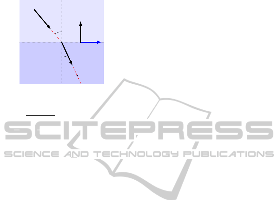
n
1
n
2
P
1
~u
1
W
P
2
~u
2
~n
~
b
P
3
θ
2
θ
1
Figure 7: Refraction of ray (P
1
,~u
1
) into (P
2
,~u
2
) under
Snell’s law.
P
2
= P
1
−
~n · (P
1
−W )
~n ·~u
1
~u
1
~u
2
=
n
1
n
2
~u
1
+
n
1
n
2
cosθ
1
− sign(cos θ
1
)cosθ
2
~n
(4)
where cosθ
1
= −~n ·~u
1
cosθ
2
=
r
1 −
n
1
n
2
2
(1 − cos
2
θ
1
) ,
given that ~n and ~u
1
have been normalized to unit
length (see Figure 7 for an illustration). Note that
no trigonometric functions need to be evaluated. The
above formula only works in the backward direction,
i.e. given the ray corresponding to an image point, we
can follow it into the second medium. However, we
are mainly interested in going the other way, comput-
ing the projection of a world point into the camera.
This is more difficult; given the world point P
3
on the
ray (P
2
,~u
2
) and camera center P
1
, determine P
2
so that
Snell’s law is satisfied (the image projection of P
3
is
then given by the in-air camera model projection of
P
2
). In previous works this has either been avoided
(Jordt-Sedlazeck and Koch, 2012), or solved by find-
ing the roots of a 12th degree polynomial (Agrawal
et al., 2012) or by numerical optimization of the back
projection (Kunz and Singh, 2008; Yau et al., 2013).
We will use a variant of the latter.
Note that the ray directions ~u
1
and ~u
2
must lie
in the same plane as the interface normal ~n; call
the normal vector of this plane ~v = ~n × (P
3
− P
1
).
This restricts the possible locations of P
2
to the line
P
2
(t) = P
0
2
+t
~
b where
~
b =~n×~v. Given P
2
(t) for some
t, we can refract and trace the ray (P
1
,P
2
(t) − P
1
)
into the second medium. At the optimal t, the ray
(P
2
(t),~u
2
(t)) will pass through P
3
. Define the signed
orthogonal distance between P
3
and the ray as d(t) =
~v ·
P
3
− P
2
(t)
×~u
2
(t). Using the intersection of the
interface plane and the straight line between P
1
and P
3
as an initial guess, we can find the zero of d(t) using
Newton’s method. For our underwater cameras, eqs.
(4) are applied twice in the backward direction, first
for the air–glass and then for the glass–water transi-
tion. Since the two interfaces are parallel, all rays
still lie in the same plane and the search remains one-
dimensional. (Yau et al., 2013) take a similar ap-
proach but minimize the error using bisection, with
inferior convergence properties.
On average over a typical range of angles, a pre-
cision of 10
−6
is reached in five iterations using for-
ward finite difference derivatives. While the method
is general and does not require the imaging plane to
be parallel with the interface(s) as in (Treibitz et al.,
2012), it is still fast and can compute the forward pro-
jection of two million points per second on a Core 2
Duo E7500 3.0 GHz computer in a C++ implemen-
tation. It is thus well-suited for use in large-scale
bundle adjustment algorithms minimizing the true im-
age re-projection error, and the algorithm is simple to
implement and easily parallelized on graphics hard-
ware. It may also be extended to the case of multiple
non-parallel interfaces, which would require a two-
dimensional search for P
2
, at some additional compu-
tational cost.
3.6 Initialization
Once we can compute the projection of any given
point into each camera, all extrinsic parameters may
be optimized through bundle adjustment if a good ini-
tialization is available. In the swimming pool case,
the positions of the cameras are easily measured by
hand or from blue-prints, and we assume these to
be known, except for the exact distance of the un-
derwater cameras to the glass pane as this number
significantly influences the refraction effects. The
thicknesses of the window panes are also considered
known, and the panes are initially assumed to be
mounted exactly flush with the pool wall.
The initial pose of the calibration object in every
frame is determined relative to the camera with the
“best” view (i.e. with the markers closest to the im-
age center), using the single-view solver above. If
the best view is an underwater camera the image will
be distorted by refraction, and solving while only ac-
counting for intrinsic camera parameters is likely to
give inaccurate results. Since the refraction effects
are actually three-dimensional in nature, the coordi-
nates cannot be exactly normalized without knowing
the depth of the markers beforehand. We settle for an
approximation where the image rays are traced into
the pool (using the initial camera and window param-
eters), and their intersections with a plane parallel to
the image plane at the expected mean depth of the cal-
ibration target are computed. The intersection points
ICPRAM2015-InternationalConferenceonPatternRecognitionApplicationsandMethods
146

are then projected back into the images, now assum-
ing there are no refraction effects, producing the mea-
surements we would have obtained had there been no
water or windows. This approximation, which as-
sumes the markers are at a known depth halfway into
the pool, is quite accurate as the depth dependence of
the correction is relatively weak, and is certainly suf-
ficient for initialization purposes.
As was noted in (Jordt-Sedlazeck and Koch,
2013), it is possible to solve exactly for the depth
of three points also in the refractive case, assuming
the camera’s pose relative to the refractive plane is
known. The camera and glass then form a gener-
alized camera (in fact, an axial camera), where the
back-projected image rays do not intersect in a com-
mon point but rather a common axis. The general-
ized 3-point pose solver (Nist
´
er, 2004) can then be
applied, which produces up to eight solutions. How-
ever, it does not exploit the fact that the points on our
calibration object are co-linear, and we have found in
experiments that our simpler solver together with the
approximation produces stabler and more accurate re-
sults under image measurement noise.
3.7 Non-linear Refinement
The bundle adjustment problem (Triggs et al., 2000)
is formulated and solved using the Ceres non-linear
least-squares solver (Agarwal et al., 2012). Due to
the relatively complex projection algorithm, numeri-
cal finite difference derivatives are used, although au-
tomatic differentiation could possibly be applied. We
allow the glass pane normals and underwater camera
distance from the glass to vary, along with all cam-
era orientations and calibration stick poses. While
the calibration thus obtained is quite accurate, the
human eye is very sensitive to discrepancies at im-
age seams which becomes obvious when rendering
stitched panoramic views. In particular, horizontal
lines on the pool wall (see Figure 10) need to match
to the pixel. To this end, we mark points in the images
along these lines, and require their back-projection in-
tersections with the pool wall to be co-linear. This
may be achieved by introducing a new variable ¯y
k
for
each line into the optimization, and adding the terms
ky
k,i
− ¯y
k
k
2
to the bundle adjustment cost function,
where y
k,i
are the vertical components of the back-
projected points lying on line k.
4 STITCHING
One goal of the calibration is to be able to stitch to-
gether images to form a panorama of the pool, or
Figure 8: Top: the initialization to the bundle adjustment
problem, where the pose of the calibration rod in each frame
has been determined from one view only (blue indicates an
underwater image was used, magenta above water). Bot-
tom: the result of optimizing over calibration object pose,
window pane normals and camera orientations. Bundle ad-
justment over the 700 poses and 1900 images took 32 sec-
onds at 7 iterations/s on a Core 2 Duo 3.0 GHz computer.
equivalently, panning shots of the swimmer. To ren-
der such a view, we define an image plane in the world
coordinate system, typically parallel to the long side
of the pool. Output pixels are sampled in a grid on
this plane, and projected into the devignetted cam-
era images to determine their color. Where images
overlap, blending is applied to smooth out the transi-
tion. For speed, projection maps for each camera can
be precomputed. Since the projection depends on the
depth of the rendering plane, separate maps are com-
puted for a discrete set of depths and then interpolated
between to match the current depth of the swimmer.
This can be efficiently implemented on graphics hard-
ware and allows us to generate full HD panning views
in real time at over 100 frames per second.
4.1 Exposure Correction
While all cameras are set to the same white balance,
exposure and gain, differences between individual
cameras are sometimes visible, particularly near the
transition edges. To minimize visual discrepancies
post-capture, we assume that the pixel value of a point
visible in two cameras simultaneously is described by
the relation γ
i
I
i
= γ
j
I
j
where γ
k
is the gain correction
for camera k and I
k
the intensity in the captured im-
age. To achieve even lighting of the stitched image,
JointUnderandOverWaterCalibrationofaSwimmerTrackingSystem
147
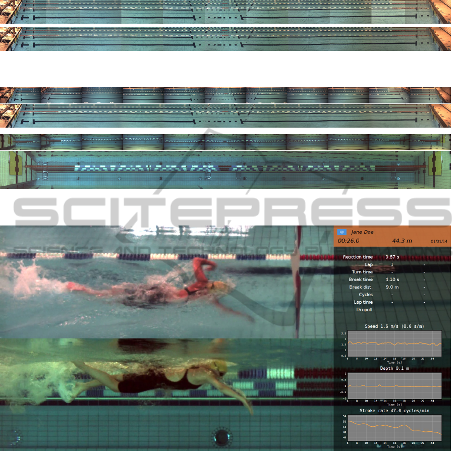
Figure 9: Exposure/gain correction. On top the uncorrected images, below each image has been multiplied with the corre-
sponding correction factor derived from equation (5). No blending has been applied at the seams.
Figure 10: The raw images captured by the camera setup along with the stitched panoramas. The lenses used are rectilinear,
the distortion effect seen in the underwater views is entirely due to refraction in the windows.
Figure 11: Still image from the final output of the swimmer tracking system. Synthetic panning views of the swimmer are
accompanied by performance statistics automatically extracted from the images.
points are sampled on the render plane and projected
into low-pass filtered images to obtain the I
k
. Each
relation above contributes a row to the linear system
.
.
.
.
.
.
.
.
.
.
.
.
.
.
.
0 I
i
0 −I
j
0
.
.
.
.
.
.
.
.
.
.
.
.
.
.
.
γ
1
.
.
.
γ
n
= 0 (5)
which can be solved for the γ in a least-squares sense
using singular value decomposition. After scaling the
gain coefficients to have unit mean, they are multi-
plied with the raw images before stitching. See Figure
9 for an illustration.
4.2 Chromatic Aberration Correction
An often ignored fact is that the indices of refraction
used in the ray-tracing equations (4) are wavelength-
dependent. However, the resulting chromatic aberra-
tion is quite pronounced even to the naked eye observ-
ing e.g. the bottom tiles of the pool through refraction
at the surface. The effect is also apparent near the
edges of our underwater images in areas of high con-
trast. By using (empirically determined) separate in-
ICPRAM2015-InternationalConferenceonPatternRecognitionApplicationsandMethods
148

Figure 12: Chromatic aberration correction. On the left,
the images were rendered using the same index of refrac-
tion of water for all channels (n = 1.333); on the right,
n
red
= 1.333, n
green
= 1.3338, n
blue
= 1.3365. Notice the
reduced rainbow effect around the edges of the black bars
(the differences are subtle so these images are best viewed
on-screen).
dices of refraction for the red, green and blue color
channels, the aberration can be almost completely
neutralized, improving the visual quality of rendered
images (see Figure 12).
The final stitched panoramas are shown in Figure
10, along with the raw images captured by each cam-
era.
5 CONCLUSION
We have developed an effective and practical proce-
dure for combined refractive and non-refractive cam-
era calibration. We have also presented an efficient
method of computing the forward projection through
refractive media, and shown how visually pleasing
stitched panoramas may be generated. The calibra-
tion data and images generated can then be used for
tracking and analyzing a swimmer’s movements in
and above the water. An example of the output of
the full system is shown in Figure 11.
REFERENCES
Agarwal, S., Mierle, K., and Others (2012). Ceres solver.
https://code.google.com/p/ceres-solver/.
Agrawal, A., Ramalingam, S., Taguchi, Y., and Chari, V.
(2012). A theory of multi-layer flat refractive geome-
try. In CVPR, pages 3346–3353. IEEE.
Chang, Y. and Chen, T. (2011). Multi-view 3d reconstruc-
tion for scenes under the refractive plane with known
vertical direction. In Proc. IEEE Int’l Conf. Computer
Vision.
Fischler, M. A. and Bolles, R. C. (1981). Random sample
consensus: A paradigm for model fitting with appli-
cations to image analysis and automated cartography.
Commun. ACM, 24(6):381–395.
Heikkila, J. and Silven, O. (1997). A four-step camera cal-
ibration procedure with implicit image correction. In
Proceedings of the 1997 Conference on Computer Vi-
sion and Pattern Recognition (CVPR ’97), CVPR ’97,
pages 1106–1, Washington, DC, USA. IEEE Com-
puter Society.
Jordt-Sedlazeck, A. and Koch, R. (2012). Refractive cal-
ibration of underwater cameras. In Fitzgibbon, A.,
Lazebnik, S., Perona, P., Sato, Y., and Schmid, C., ed-
itors, Computer Vision – ECCV 2012, volume 7576 of
Lecture Notes in Computer Science, pages 846–859.
Springer Berlin Heidelberg.
Jordt-Sedlazeck, A. and Koch, R. (2013). Refractive
structure-from-motion on underwater images. In
Computer Vision (ICCV), 2013 IEEE International
Conference on, pages 57–64.
Kang, L., Wu, L., and Yang, Y.-H. (2012). Two-view un-
derwater structure and motion for cameras under flat
refractive interfaces. In Fitzgibbon, A. W., Lazebnik,
S., Perona, P., Sato, Y., and Schmid, C., editors, ECCV
(4), volume 7575 of Lecture Notes in Computer Sci-
ence, pages 303–316. Springer.
Kunz, C. and Singh, H. (2008). Hemispherical refrac-
tion and camera calibration in underwater vision. In
OCEANS 2008, pages 1–7. IEEE.
Nist
´
er, D. (2004). A minimal solution to the generalised
3-point pose problem. In CVPR (1), pages 560–567.
Treibitz, T., Schechner, Y. Y., Kunz, C., and Singh, H.
(2012). Flat refractive geometry. IEEE Transac-
tions on Pattern Analysis and Machine Intelligence,
34(1):51–65.
Triggs, B., Mclauchlan, P., Hartley, R., and Fitzgibbon, A.
(2000). Bundle adjustment – a modern synthesis. In
Vision Algorithms: Theory and Practice, LNCS, pages
298–375. Springer Verlag.
Yau, T., Gong, M., and Yang, Y.-H. (2013). Underwa-
ter camera calibration using wavelength triangulation.
In Computer Vision and Pattern Recognition (CVPR),
2013 IEEE Conference on, pages 2499–2506.
Zhang, Z. (1999). Flexible camera calibration by viewing
a plane from unknown orientations. In Computer Vi-
sion (ICCV), 1999 IEEE International Conference on,
pages 666–673.
JointUnderandOverWaterCalibrationofaSwimmerTrackingSystem
149
