Thompson Sampling in the Adaptive Linear Scalarized

Multi Objective Multi Armed Bandit

Saba Q. Yahyaa, Madalina M. Drugan and Bernard Manderick

Department of Computer Science, Vrije Universiteit Brussel, Pleinlaan 2, 1050 Brussels, Belgium

Keywords:

Multi-armed Bandit Problems, Multi-objective Optimization, Linear Scalarized Function, Scalarized Function

Set, Thompson Sampling Policy.

Abstract:

In the stochastic multi-objective multi-armed bandit (MOMAB), arms generate a vector of stochastic normal

rewards, one per objective, instead of a single scalar reward. As a result, there is not only one optimal arm,

but there is a set of optimal arms (Pareto front) using Pareto dominance relation. The goal of an agent is to

ﬁnd the Pareto front. To ﬁnd the optimal arms, the agent can use linear scalarization function that transforms

a multi-objective problem into a single problem by summing the weighted objectives. Selecting the weights is

crucial, since different weights will result in selecting a different optimum arm from the Pareto front. Usually,

a predeﬁned weights set is used and this can be computational inefﬁcient when different weights will optimize

the same Pareto optimal arm and arms in the Pareto front are not identiﬁed. In this paper, we propose a

number of techniques that adapt the weights on the ﬂy in order to ameliorate the performance of the scalarized

MOMAB. We use genetic and adaptive scalarization functions from multi-objective optimization to generate

new weights. We propose to use Thompson sampling policy to select frequently the weights that identify new

arms on the Pareto front. We experimentally show that Thompson sampling improves the performance of the

genetic and adaptive scalarization functions. All the proposed techniques improves the performance of the

standard scalarized MOMAB with a ﬁxed set of weights.

1 INTRODUCTION

Multi-Objective Optimization (MOO) problem with

conﬂicting objectives is present everywhere in the

real-world. For instance, in shipping ﬁrm, the con-

ﬂicting objectives could be consist of the shipping

time and the cost. At the same time, shorten shipping

time is needed in order to improve customer satisfac-

tion, while also reducing the number of used ships to

reduce the operating cost. It is obvious that adding

more ships will reduce the needed shipping time but

will increase the operating cost. The goal of the MOO

with conﬂicted objectives is to tradeoff the conﬂicting

objectives. The Multi-Objective Multi-Armed Ban-

dit (MOMAB) problem (Drugan and Nowe, 2013; S.

Q. Yahyaa and Manderick, 2014b) is the simplest ap-

proach to representing the MOO problem.

MOMAB problem is a sequential stochastic learn-

ing problem. At each time step t, an agent pulls one

arm i from an available set of arms A and receives a

reward vector r

from the arm i with D dimensions

(or objectives) as feedback signal. The reward vec-

tor is drawn from a probability distribution vector,

for example from a normal probability distribution

N(µ

,σ

), where µ

is the true mean vector and σ

the covariance matrix parameters of the arm i. The

reward vector r

that the agent receives from the arm

i is independent from all other arms and independent

from the past reward vectors of the selected arm i.

Moreover, the mean vector of the arm i has indepen-

dent D distributions, i.e. σ

is a diagonal covariance

matrix. We assume that the true mean vector and co-

variance matrix of each arm i are unknown parame-

ters to the agent. Thus, by drawing each arm i, the

agent maintains estimations of the true mean vector

and the diagonal covariance matrix (or the variance

vector) which are known as

and

, respectively.

The MOMAB problem has a set of Pareto optimal

arms (Pareto front) A

∗

, that are incomparable, i.e. can

not be classiﬁed using a designed partial order rela-

tions (Zitzler and et al., 2002). The agent has to ﬁg-

ure out the optimal arms to minimize the total Pareto

loss of not pulling the optimal arms. At each time

step t, the Pareto loss (or Pareto regret) is the distance

between the set mean of Pareto optimal arms and the

mean of the selected arm (Drugan and Nowe, 2013).

Yahyaa S., Drugan M. and Manderick B..

Thompson Sampling in the Adaptive Linear Scalarized Multi Objective Multi Armed Bandit.

DOI: 10.5220/0005184400550065

In Proceedings of the International Conference on Agents and Artiﬁcial Intelligence (ICAART-2015), pages 55-65

ISBN: 978-989-758-074-1

 2015 SCITEPRESS (Science and Technology Publications, Lda.)

Thus, the total Pareto regret is the cumulativesumma-

tion of the Pareto regret over t time steps.

The Pareto front A

∗

can be found for example,

by using linear scalarized function (f) (Eichfelder,

2008). Linear scalarized function is simple and in-

tuitive. Given a predeﬁned set weight w

w, the linear

scalarized function f weighs each value of the mean

vector of an arm i, converts the multi-objective space

to a single-objective one by summing the weighted

mean values and selects the optimal arm i

∗

that has

the maximum scalarized function. However, solving

a multi-objective optimization problem means ﬁnd-

ing the Pareto front A

∗

. Thus, we need various lin-

ear scalarized functions F

F, each scalarized function

, f

∈ F

F, s = 1,·· · ,S has a corresponding set of

weight w

, to generate the variety of elements belong-

ing to the Pareto front. The predeﬁned total weight

setW

W, W

W = {w

,· ·· ,w

} is uniformly random spread

sampling in the weighted space (Das and Dennis,

1997). However, there is no guarantee that the to-

tal weight set W

W can ﬁnd all the optimal arms in the

Pareto front A

∗

. To improve the performance of the

linear scalarized function (S. Q. Yahyaa and Mander-

ick, 2014a) have used Knowledge Gradient (KG) pol-

icy (I. O. Ryzhov and Frazier, 2011) in the MOMAB

problem, resulting Linear Scalarized Knowledge Gra-

dient Function (LS-KG-F).

In this paper, we improve the performance of

the linear scalarized knowledge gradient function LS-

KG-F by introducing techniques from multi-objective

optimization that redeﬁne the weights for the weight

set w

w. We either generate a new weight set w

w by

using genetic operators that change the weights di-

rectly (Drugan, 2013) or adapt the weights by using

the arms in the Pareto front like in (J. Dubois-Lacoste

and Stutzle, 2011). We propose also the Thompson

sampling policy (Thompson, 1933) to select from the

total weight set W

W, the weight set w

w that identiﬁes a

larger set of optimal arms from the Pareto front A

∗

The rest of the paper is organized as follows:

In Section 2 we introduce the multi-objective multi-

armed bandit problem. In Section 3 we present the

linear scalarized functions and the scalarized multi-

objective bandits algorithm. In Section 4 we intro-

duce algorithms to determine the weight set, the stan-

dard, the adaptive and the genetic algorithms. In

Section 5 we introduce the adaptive scalarized multi-

objective bandits algorithm that uses Thompson sam-

pling policy to select the appropriate weight set. In

Section 6, we describe the experiments set up fol-

lowed by experimental results. Finally, we conclude

and discuss future work.

2 MULTI OBJECTIVE MULTI

ARMED BANDITS PROBLEM

Let us consider the MOMABs problems with |A| ≥ 2

arms and with independent D objectives per arm. At

each time step t, the agent selects one arm i and

receives a reward vector r

. The reward vector r

is drawn from a corresponding normal probability

distribution N(µ

,σ

) with unknown mean parameter

vector µ

, µ

= [µ

,· ·· ,µ

]

and unknown variance

parameter vector σ

, σ

= [σ

2,1

,· ·· ,σ

2,D

]

, where T

is the transpose. Thus, by drawing each arm i, the

agent maintains estimate of the mean parameter vec-

tor

and the variance

parameter vector, and com-

putes the number of times N

arm i is drawn. The

agent updates the estimated mean ˆµ

, the estimated

variance

2,d

of the selected arm i in each objective

d,d ∈ D and the number of times N

arm i has been

selected as follows (Powell, 2007):

i+1

= N

+ 1 (1)

ˆµ

i+1

= (1−

i+1

) ˆµ

i+1

t+1

(2)

2,d

i+1

− 2

i+1

− 1

2,d

i+1

t+1

− ˆµ

)

(3)

where N

i+1

is the updated number of times arm i has

been selected, ˆµ

i+1

is the updated estimated mean,

and

2,d

i+1

is the updated estimated variance of the arm

i in the objective d and r

t+1

is the observed reward of

the arm i in the objective d.

When the objectives are conﬂicting with one an-

other then the mean component µ

of arm i corre-

sponding with objective d, d ∈ D, can be better than

the component µ

of another arm j but worse if we

compare the components for another objective d

′

> µ

but µ

′

< µ

′

for objectives d and d

′

, respec-

tively. The agent has a set of optimal arms (Pareto

front) A

∗

which can be found by the Pareto dominance

relation (or Pareto partial order relation).

The Pareto dominance relation ﬁnds the Pareto

front A

∗

directly in the multi-objectiveMO space (Zit-

zler and et al., 2002). It uses the following relations

between the mean vectors of two arms. We use i and

j to refer to the mean vector (estimated mean vector

or true mean vector) of arms i and j, respectively:

Arm i dominates or is better than j, i ≻ j, if there

exists at least one objective d for which i

≻ j

and

for all other objectives d

′

we have i

′

 j

′

. Arm i is

incomparable with j, i k j, if and only if there exists

at least one objective d for which i

≻ j

and there

exists another objective d

′

for which i

′

≺ j

′

. Arm i

is not dominated by j, j ⊁ i, if and only if there exists

ICAART2015-InternationalConferenceonAgentsandArtificialIntelligence

at least one objective d for which j

≺ i

. This means

that either i ≻ j or i k j.

Using the above relations, Pareto front A

∗

⊂ A

be the set of arms that are not dominated by all other

arms. Moreover, the optimal arms in A

∗

are incompa-

rable with each other.

In the MOMAB, the agent has to ﬁnd the Pareto

front A

∗

, therefore, the performance measure is the

Pareto regret (Drugan and Nowe, 2013). The Pareto

regret measure (R

Pareto

) measures the distance be-

tween a mean vector of an arm i that is pulled at

time step t and the Pareto front A

∗

. Pareto regret

Pareto

is calculated by ﬁnding ﬁrstly the virtual dis-

tance dis

∗

. The virtual distance dis

∗

is deﬁned as

the minimum distance that is added to the mean

vector of the pulled arm µ

at time step t in each

objective to create a virtual mean vector µ

∗

, µ

∗

+ ε

∗

that is incomparable with all the arms in

Pareto set A

∗

, i.e. µ

∗

||µ

∀

i∈A

∗

. Where ε

∗

is a vec-

tor, ε

∗

= [dis

∗,1

,· ·· ,dis

∗,D

]

. Then, the Pareto regret

Pareto

, R

Pareto

= dis(µ

,µ

∗

) = dis(ε

∗

0) is the dis-

tance between the mean vector of the virtual arm µ

∗

and the mean vector of the pulled arm µ

at time step

t, where dis, dis(µ

,µ

∗

) = (

∑

d=1

(µ

∗,d

− µ

)

(1/2)

the Euclidean distance. Thus, the regret of the Pareto

front is 0 for optimal arms, i.e. the mean of the opti-

mal arm coincides itself.

3 THE SCALARIZED

MULTI-OBJECTIEVE BANDITS

Linear scalarization function converts the multi-

objective into single-objective optimization (Eich-

felder, 2008). However, solving a multi-objective op-

timization problem means ﬁnding the Pareto front A

∗

Thus, we need a set of scalarized functions F

F, F

F =

{ f

,· ·· , f

} to generate a variety of elements

belonging to the Pareto front A

∗

. Each scalarized

function f

, f

∈ F

F has a corresponding predeﬁned

set of weight w

, w

∈ W

W, whereW

W = (w

,· ·· ,w

The linear scalarization function assigns to each

value of the mean vector of an arm i a weight w

and the result is the sum of these weighted mean

values. Given a predeﬁned set of weights w

, w

,· ·· ,w

) such that

∑

d=1

= 1, the linear scalar-

ized across mean vector is:

(µ

) = w

+ ··· + w

(4)

where f

(µ

) is a linear scalarized function s, s ∈ S

over the mean vector µ

of the arm i. After transform-

ing the multi-objective problem to a single-objective

problem, the linear scalarized function f

selects the

arm i

∗

that has the maximum linear scalarized func-

tion value:

∗

= argmax

1≤i≤A

(µ

)

The linear scalarization is very popular because of

its simplicity. However, it can not ﬁnd all the optimal

arms in the Pareto front A

∗

(Das and Dennis, 1997).

To improve the performance of the linear scalar-

ized function, (S. Q. Yahyaa and Manderick, 2014b)

have extended Knowledge Gradient (KG) policy (I.

O. Ryzhov and Frazier, 2011) to the MOMAB prob-

lem, resulting linear scalarization function knowledge

gradient. (S. Q. Yahyaa and Manderick, 2014b) have

proposed two variants of linear scalarized KG, lin-

ear saclarized KG across arms (LS1-KG) and linear

saclarized KG across dimensions (LS2-KG). Since

LS1-KG performs better than LS2-KG, we will use

linear scalarized KG across arms LS1-KG.

The linear scalarized-KG across arms (LS1-

KG) converts the multi-objective estimated mean

= [ˆµ

,· ·· , ˆµ

]

and estimated variance

[

2,1

,· ·· ,

2,D

]

of each arm to one-objective, then

computes the corresponding bound (or term) ExpB

At each time step t, LS1-KG weighs both the esti-

mated mean vector

and estimated variance vector

of each arm i, converts the multi-objective vec-

tors to one-objective values by summing the elements

of each vector. Thus, we have one-objective multi-

armed bandits problem. The KG policy calculates

for each arm, a bound which depends on all avail-

able arms and selects the arm that has the maximum

estimated mean plus the bound. The LS1-KG is as

follows:

eµ

= f

(

) = w

ˆµ

+ ··· + w

ˆµ

∀

(5)

= f

(

) = w

2,1

+ ··· + w

2,D

∀

(6)

∀

(7)





−|

eµ

− max

j6=i, j∈A

eµ





∀

(8)

where f

is a linear scalarization function that has a

predeﬁned set of weight w

= (w

,· ·· ,w

), eµ

, and

are the modiﬁed estimated mean, and the modi-

ﬁed estimated variance of an arm i, respectively which

are one-objective values and

is the modiﬁed Root

Mean Square Error (RMSE) of an arm i. The v

the KG index of an arm i. The function g(ζ), g(ζ) =

ζΦ(ζ) + φ(ζ), where Φ, and φ are the cumulative

distribution, and the density of the standard normal

density N(0,1), respectively. Linear scalarized-KG

ThompsonSamplingintheAdaptiveLinearScalarizedMultiObjectiveMultiArmedBandit

across arms selects the optimal arm i

∗

according

to:

∗

= argmax

i=1,···,|A|

(eµ

+ ExpB

) (9)

= argmax

i=1,···,|A|

(eµ

+ (L− t) ∗ |A|D ∗ v

) (10)

where ExpB

is the bound of arm i, |A| is the number

of arms, D is the number of objectives, L is the hori-

zon of an experiments, i.e. length of trajectories and t

is the current time step.

The algorithm. The pseudocode of the Scalarized

Multi-objectieve Multi-Armed Bandit (SMOMAB)

algorithm is given in Figure 1. The linear scalarized-

KG across arms LS1-KG function is f. The scalar-

ized function set isF

F = ( f

,· ·· , f

), where each LS1-

KG function f

has a predeﬁned weight set, w

1,s

,· ·· ,w

D,s

) and the number of scalarized function

is |S|, |S| = D+ 1.

The algorithm in Figure 1 plays each arm for each

scalarized function s, Initial plays (step: 2)

. N

is the

number of times the scalarized function s is pulled and

is the number of times the arm i under the scalar-

ized function s is pulled. (r

)

is the reward of the

pulled arm i under the scalarized function s which is

drawn from a normal distribution N(µ

µ,σ

), whereµ

µ is

the unknown true mean vector and σ

is the unknown

true variance vector of the reward. (

)

and (

)

are the estimated mean and standard deviation vectors

of the arm i under the scalarized function s, respec-

tively. After initial playing, the algorithm chooses

uniformly at random one of the scalarized function

s (step: 4). The algorithm determines the correspond-

ing weight set w

such that

∑

d=1

d,s

= 1 (step: 5).

The weight set w

can be speciﬁed by using stan-

dard algorithm (Das and Dennis, 1997), adaptive al-

gorithm (J. Dubois-Lacoste and Stutzle, 2011), or ge-

netic algorithm (Drugan, 2013), we refer to Section 4

for more details. If the SMOMAB algorithm uses the

standard algorithm to set the weights, then the total

weight set W

W = (w

,· ·· ,w

) is ﬁxed until the end of

playing L steps. However, if the SMOMAB algorithm

uses the adaptive or the genetic algorithm, then the

total weight setW

W = (w

,· ·· ,w

) will change at each

time step. The SMOMAB algorithm uses the prede-

ﬁned total weight set W

W till the end of playing Initial

steps, then at each time step the adaptive and the ge-

netic algorithms generate new weights. The algorithm

selects the optimal arm (i

∗

)

that maximizes the LS1-

KG function (step: 6) and simulates the selected arm

∗

)

to observe the reward vector (r

∗

)

(step: 7). The

We use s to refer the scalarized function f

that has a

predeﬁned weight set w

= (w

,·· · ,w

,·· · , w

estimated mean vector (

∗

)

, estimated standard de-

viation vector (

∗

)

, and the number N

∗

of the se-

lected arm and the number of the pulled scalarized

function N

are updated (step: 8). Finally, the al-

gorithm computes the Pareto regret (step: 9). This

procedure is repeated until the end of playing L steps

which is the horizon of an experiment.

Note that, the algorithm in Figure 1 is an adapted

version of the scalarized MOMABs from (Drugan and

Nowe, 2013), but here the reward is drawn from nor-

mal distribution and the weight set w

is determined.

Input:

Horizon of an experiment

;number

of arms

|A|

;number of objectives

;number of

scalarized functions

|S| = D+ 1

;reward vector

r ∼ N(µ

µ,σ

)

Initialize:

Total Weight set

W = (w

,· ··,w

D+1

)

For each scalarized function

s = 1

Play: each arm

Initial

steps

Observe:

)

Update:

← N

+ 1

;

← N

+ 1

;

(ˆµ

)

;

(

)

End

Repeat

4. Select a function

uniformly at random

5. Compute the weight set

← Weight

6. Select the optimal arm

∗

)

that maximizes

the scalarized function

7. Observe: reward vector

∗

)

∗

)

= ([r

∗

,· ··, r

∗

]

)

8. Update:

(

∗

)

;

(

∗

)

;

∗

← N

∗

+ 1

;

← N

+ 1

9. Compute: Pareto regret

10.

Until L

11. Output: Pareto regret

Figure 1: The scalarized multi-objective multi-armed bandit

(SMOMAB) algorithm.

4 ADAPTIVE WEIGHTS FOR

THE SCALARIZED MOMAB

In this section, we provide different algorithms to

identify the weight set w

Fixed set of weights. The standard algo-

rithm (Das and Dennis, 1997) deﬁnes a ﬁxed to-

tal weight set W

W, W

W = (w

,· ·· ,w

) that is

uniformly random spread sampling in the weighted

space. For example, the bi-objective multi-armed

bandit with number of scalarized function |S|. The

weight w

1,s

of the scalarized function s in the objec-

tive d, d = 1 is set to 1−

s−1

|S|−1

and the weight w

2,s

the scalarized function s in the objective d, d = 2 is

set to 1− w

1,s

Note that, this algorithm performs a uniform sam-

pling in the weight space. However, there is no

ICAART2015-InternationalConferenceonAgentsandArtificialIntelligence

guarantee that the resulting arms will give a uni-

form spread in the objective space. The weight set

, w

∈ W

W is sequentially ordered, therefore, when

the scalarized MOMAB algorithm (the algorithm in

Figure 1) is stopped prematurely, it will not have sam-

pled all the part of the weight space, possibly leaving

a part of the Pareto front A

∗

undiscovered.

Adaptive Direction. The adaptive algorithm from

(J. Dubois-Lacoste and Stutzle, 2011) takes into ac-

count the shape of the Pareto front A

∗

in order to

obtain a well-spread set of the non-dominated arms.

For a scalarized function s, this algorithm deﬁnes a

norm (Euclidean distance) to specify the largest gap

in the coverage of the Pareto front A

∗

. The largest gap

is the gap between the maximum norm max

i∈A

and the minimum norm min

i∈A

|| of the estimated

mean

of an arm i, i ∈ A under the scalarized func-

tion s. For example, the bi-objective multi-armed

bandit with scalarized function s. The adaptive new

weight w

1,s

of the objective d, d = 1 is perpendic-

ular to the segment deﬁned by the maximum arm

max

, i

max

= argmax

i∈A

|| and the minimum arm

arm i

min

, i

min

= argmin

i∈A

|| in the objective space,

that is:

1,s

ˆµ

2,s

max

− ˆµ

2,s

min

ˆµ

2,s

max

− ˆµ

2,s

min

+ ˆµ

1,s

min

− ˆµ

1,s

max

where ˆµ

2,s

max

and ˆµ

2,s

min

are the estimated mean of the

arms i

max

and i

min

in the objective 2 under scalarized

function s, respectively . And, ˆµ

1,s

max

and ˆµ

1,s

min

are the

estimated mean of the arms i

max

and i

min

in the objec-

tive 1 under scalarized function s, respectively. The

new weight w

2,s

of the second objective d = 2 un-

der scalarized function s is set to 1 − w

1,s

. Note that,

for number of objectives D > 2, the weight w

in the

objective d = 1 is calculated by using the estimated

mean of the objectives d = 1 and d = 2. The weight

in the objective d = 2 is calculated by using the es-

timated mean of the objectives d = 2 and d = 3, and

so on. While the weight w

in the objective D is set

to 1− (w

+ ··· + w

D−1

This algorithm deﬁnes new weights based on the

shape of the Pareto front. Therefore, if the shape of

the Pareto front is irregular, then the new weight will

not discover all the optimal arms in the Pareto front.

This operator adapt the weights of only two objectives

at the time.

Genetic Operators. The scalarized local search al-

gorithm (Drugan, 2013) generates new weights for

scalarized function s using real-coded genetic oper-

ators. The new weights are different from the parent-

ing weights, therefore, it could explore the parts of the

Pareto front A

∗

that are undiscovered.

The mutation operator, mutates each weight of a

scalarization function independently using a normal

distribution. The recombination operator generates a

new weight w

w from two or more scalarized functions,

each scalarized function has a predeﬁned weight set

= (w

,· ·· ,w

). The translation recombination

operator translates the main set of scalarized function

S with a normally distributed variable. The rotation

recombination operator, considers that the scalarized

functions S are positioned on a S-dimensional hyper-

sphere. The generated new scalarized function s also

belongs to this hypersphere around the main scalar-

ized functions S, that is rotated with a small normally

distributed angle. For more details, we refer to (Dru-

gan and Thierens, 2010).

Since the mutation operator is the easiest one to

implement, we will use it in our comparison. Given

the weight setw

(t) of the scalarized function s at time

step t, the mutated new set of weight w

(t + 1) at time

step t + 1 is calculated as follows;

(t + 1) = w

(t) + I

where I

I is a diagonal matrix of size D × D with nor-

mally distributed variables and 1

1 is a vector of size

D with 1 variables. After calculating the new weight

set w

(t + 1), we can either replace the old weight set

(t) with the new weight set, i.e. w

(t) ← w

(t + 1)

(mutation) or at each time step t, we generate new set

of weight that is independent from the previous one

(mutation without replacement).

5 THOMPSON SAMPLING IN

THE SCALARIZED MOMAB

ALGORITHM

In this section, we design an algorithm that frequently

selects the appropriated scalarized function set of

weights w

, w

∈ W

W, where the total weight set W

W is

either determined by using standard algorithm, adap-

tive algorithm or genetic algorithm. The appropriate

scalarized function is the one that improves the per-

formance of the algorithm by identifying new Pareto

optimal arms.

In the Bernoulli one-objective,Multi-Armed Ban-

dits (MABs), the reward is a stochastic scalar value,

and there is only one optimal arm. The reward r

, r

∼

B(p

) for an arm i is either 0, or 1 and generated from

a Bernoulli distribution B with unknown probability

of success p

. The goal of an agent is to minimize the

loss of not pulling the best arm i

∗

over L time steps.

The loss (or the total regret) is R

= Lp

∗

−

∑

t=1

(t),

where p

∗

= max

i=1,···,A

is the probability of suc-

ThompsonSamplingintheAdaptiveLinearScalarizedMultiObjectiveMultiArmedBandit

cess of the best arm i

∗

, and p

is the probability of

success of the selected arm i at time step t. To mini-

mize the total regret, at each time step t, the agent has

to trade-off between selecting the optimal arm i

∗

(ex-

ploitation) to minimize the regret

and selecting one

of the non-optimal arm i to increase the conﬁdence in

the estimated probability of success ˆp

, ˆp

/(α

+ β

)

of the arm i (exploration). Where α

is the number of

successes (the number of receiving reward equals 1)

and β

is the number of failures (the number of receiv-

ing reward equals 0) of the arm i.

Thompson Sampling Policy. (Thompson, 1933) as-

signs to each arm i, i ∈ A a random probability of

selection P

to trade-off between exploration and ex-

ploitation. The random probability of selection P

each arm i is generated from Beta distribution, i.e.

= Beta(α

,β

), where α

is the number of successes

and β

is the number of failures of the arm i. The ran-

dom probability of selection P

of an arm i depends

on the performance of the arm i, i.e. the unknown

probability of success p

of the arm i. It will be high

value if the arm i has high probability of success p

value. With Bayesian priors on the Bernoulli proba-

bility of success p

of each arm i, Thompson sampling

assumes initially the number of successes, α

and the

number of failures, β

for each arm i is 1. At each

time t, Thompson sampling samples the probability

of selection P

for each arm i, i ∈ A (the probability

that an arm i is optimal) from Beta distribution, i.e.

= Beta(α

,β

). Beta distribution generates random

values, therefore, probably, at time step t, the optimal

arm i

∗

, i

∗

= argmax

i∈A

has high probability of se-

lection P

∗

, while at time step t +1 the suboptimal arm

j, j ∈ A, j 6= i

∗

has high probability of selection P

Thompson sampling selects the optimal arm i

∗

that has the maximum probability of selection P

∗

i.e. i

∗

= argmax

i∈A

and observes the reward r

∗

If r

∗

= 1, then Thompson sampling updates the num-

ber of successes α

∗

= α

∗

+ 1 for the arm i

∗

. As

a result, the estimated probability of success ˆp

∗

the arm i

∗

will increase. If r

∗

= 0, then Thomp-

son sampling updated the number of failures β

∗

+1 for the arm i

∗

. As a result, the estimated prob-

ability of success ˆp

∗

of the arm i

∗

will decrease.

Since, Thompson sampling is very easy to imple-

ment, we will use it to select the scalarized function

s, s ∈ S. We assume that each scalarized function s

has unknown probability of success p

and when we

select s, we either receive reward 1 or 0. We call

the algorithm that uses Thompson sampling to select

the weight set ”Adaptive Scalarized Multi-Objective

Multi-Armed Bandit” (adaptive-SMOMAB). Note

At each time step t, the regret equals p

∗

− p

(t).

that, adaptive-SMOMAB uses Thompson sampling to

select the weight set, while scalarized multi-objective

multi-armed bandit (MOMAB) selects uniformly at

random one of the weight set w

, w

∈ W

The Adaptive-SMOMAB Algorithm. As in the case

of MABs, Thompson sampling uses random of beta

distribution Beta(α

,β

) to assign a probability of se-

lection P

for each scalarized function s. Where α

is the number of successes of the scalarized function

s and β

is the number of failures of the scalarized

function s. We consider that each scalarized func-

tion s has unknown probability of success p

and by

playing each scalarized function s, we can estimate

the corresponding probability of success. At each

time step t, we maintain value V

(t) for each scalar-

ized function s, where V

(t) = max

i∈A

((

)

) is the

value of the optimal arm i

∗

, i

∗

= argmax

i∈A

((

)

under scalarized function s and (

)

is the estimated

mean vector of the arm i under the scalarized func-

tion s. If we select the scalarized function s at time

step t and the value of this scalarized function V

(t) is

greater or equal than the value at the previous selec-

tion, V

(t) ≥ V

(t − 1), then this scalarized function s

performs well because it has the ability to select the

same optimal arm or to select another optimal arm

that has higher value. Otherwise, the scalarized func-

tion s does not perform well.

The pseudocode of the adaptive-SMOMAB algorithm

is given in Figure 2. The linear scalarized-KG across

arms LS1-KG function f is used to convert the multi-

objective to a single one. The number of scalarized

function is |S|, |S| = D + 1, where D is the number

of objectives. The horizon of an experiment is L

steps. The algorithm in Figure 2 plays each arm for

each scalarized function s, Initial plays. The scalar-

ized function set is F

F = ( f

,· ·· , f

|S|

), each scalarized

function s has a corresponding predeﬁned weight set,

= (w

1,s

,· ·· ,w

D,s

). N

is the number of times the

scalarized function s is pulled and N

is the number

of times the arm i under the scalarized function s is

pulled. (r

)

is the reward vector of the pulled arm i

under the scalarized function s which is drawn from a

normal distribution N(µ

µ,σ

), whereµ

µ is the true mean

vector andσ

is the true variance vector of the reward.

(

)

and (

)

are the estimated mean and standard

deviation vectors of the arm i under the scalarized

function s, respectively. V

, V

= max

i∈A

((

)

) is

the value of each scalarized function s after playing

each arm i Initial steps, where f

((

)

) is the value

of the LS-KG for the arm i under scalarized function

s. The number of successes α

, and the number of

failures β

for each scalarized function s are set to 1

as (Thompson, 1933), therefore, the estimated proba-

bility ˆp

, ˆp

/(α

+ β

) of success is 0.5. The prob-

ICAART2015-InternationalConferenceonAgentsandArtificialIntelligence

Input:

Horizon of an experiment

;number

of arms

|A|

;number of objectives

;number of

scalarized functions

|S| = D+ 1

;reward vector

r ∼ N(µ

µ,σ

)

Initialize:

Total wight set

W = (w

,· ··,w

D+1

)

For each scalarized function

s = 1

|S|

Play: each arm

Initial

steps

Observe:

)

Update:

← N

+ 1

;

← N

+ 1

(

)

;

(

)

Compute:

(t) = max

1≤ i≤ A

((ˆµ

ˆµ

)

Set:

= 1

;

= 1

;

ˆp

= 0.5

;

|S|

End

Repeat

4. For each scalarized function

s = 1,· ··, S

5. Sample

from Beta

(α

,β

)

6. End for

∗

= argmax

8. Compute: the new weight set

∗

← Weight

9. Select: the optimal arm

∗

that maximizes

scalarized function

∗

that has

the new weight set

∗

10. Compute:

∗

(t) = max

1≤ i≤ A

∗

((ˆµ

ˆµ

)

∗

)

11. If

∗

(t) ≥ V

∗

(t −1)

12.

∗

= α

∗

+ 1

13. Else

14.

∗

= β

∗

+ 1

15. End

16.

∗

(t −1) ← V

∗

(t)

17. Observe: reward vector

∗

)

∗

= ([r

∗

,· ··, r

∗

]

)

∗

18. Update:

(

∗

)

∗

;

(

∗

)

∗

;

∗

← N

∗

+ 1

;

∗

← N

∗

+ 1

19. Compute: Pareto regret

20.

Until L

21.

Output:

Pareto regret

Figure 2: Adaptive Scalarized MOMAB.

ability of selection P

each scalarized function s is

|S|

(step: 2).

After initial playing, the algorithm computes the

probability of selection P

of each scalarized function

s, the probability of selection P

is sampled from beta

distribution Beta(α

,β

)(step: 4). The algorithm se-

lects the optimal scalarized function s

∗

, the one that

has a max probability of success (step: 7). The al-

gorithm determines the weight set w

∗

for the optimal

scalarized function s

∗

(step: 8). The weight set w

∗

is determined either by using adaptive algorithm, ge-

netic algorithm or standard algorithm, Section 4. The

algorithm selects the optimal arm i

∗

under the optimal

scalarized function s (step: 9) and computes the value

of the optimal scalarized function s

∗

(step: 10) which

is the value of the optimal arm i

∗

. If the value V

∗

(t)

of the optimal scalarized function s

∗

at time step t, is

greater or equal than the value of the of the optimal

scalarized function s

∗

at time step t − 1, then the opti-

mal scalarized function s

∗

performs well. The number

of successes α

∗

is increased. Other wise, the number

of failures β

∗

is increased (steps: 11-15). Then, the

algorithm updates the value V

∗

of the optimal scalar-

ized function s

∗

(step: 16). The algorithm simulates

the optimal arm i

∗

of the optimal scalarized function

∗

, observes the corresponding reward vector (r

∗

)

∗

and updates the estimated mean vector (ˆµ

ˆµ

∗

)

∗

, the es-

timated standard deviation vector (

∗

)

∗

of the arm

∗

and updates the number N

∗

of the selected arm

and the number of the pulled scalarized function N

∗

(steps: 17-18). Finally, the algorithm computes the

Pareto regret (step: 19). This procedure is repeated

until the end of playing L steps.

Note that, if the adaptive-SMOMAB algorithm

uses the standard algorithm to set the weights, then

the total weight set W

W = (w

,· ·· ,w

) is ﬁxed un-

til the end of playing L steps. However, if the

adaptive-SMOMAB algorithm uses the adaptive or

the genetic algorithm, then the total weight set W

W =

,· ·· ,w

) will change at each time step. The

adaptive-SMOMAB algorithm uses a predeﬁned to-

tal weight set W

W till the end of playing Initial steps,

then at each time step the adaptive and the genetic al-

gorithms generate new weights.

6 EXPERIMENTS

In this section, we ﬁrstly compare the performance of

the adaptive scalarized multi-objective, multi-armed

bandit (adaptive-SMOMAB)algorithm, the algorithm

in Figure 2 and the performance of the scalarized

multi-objective multi-armed bandit (SMOMAB) al-

gorithm, the algorithm in Figure 1. We use the

genetic, the adaptive, and the standard algorithms,

Section 4 to set the weight set w

for each linear

scalarized knowledge gradient across arms (LS1-KG)

s. Secondly, we experimentally compare the stan-

dard, the adaptive and the genetic algorithms, using

the adaptive-SMOMAB algorithm. The performance

measures are:

1. The Pareto regret, Section 2 at each time step t

which is the average of M experiments.

2. The cumulative Pareto regret, Section 2 at each

time step t which is the average of M experiments.

The number of experiments M is 1000. The hori-

zon of each experiment L is 1000. The reward vectors

of each arm i are drawn from corresponding normal

distribution N(µ

,σ

i,r

) where µ

= [µ

,· ·· ,µ

]

is the

true mean vector and σ

i,r

= [σ

i,r

,· ·· ,σ

i,r

]

is the true

ThompsonSamplingintheAdaptiveLinearScalarizedMultiObjectiveMultiArmedBandit

standard deviation vector of the reward of the arm i.

The true means and the true standard deviations of

arms are unknown parameters to the agent. The LS1-

KG needs the estimated variance

for each arm i,

therefore, each arm is played initially 2 times which

is the minimum number to estimate the variance.

At each time step t, the mutation operator mu-

tates the weight set w

(t) of each scalarized function

s at time step t independently using a normal distri-

bution N(µ, σ

) to generate new weight set w

(t + 1),

we set the mean µ to 0 and the variance σ

to 0.05

as (Drugan, 2013). We can either replace the old

weight w

(t) set with the new weight set w

(t + 1),

i.e. w

(t) ← w

(t + 1) or at each time step t, we gen-

erate new set of weight that is independent from the

previous one. We compare the two different setting

and we ﬁnd out that the replacement setting performs

better, therefore, we use this in our comparison.

6.1 Bi-Objective

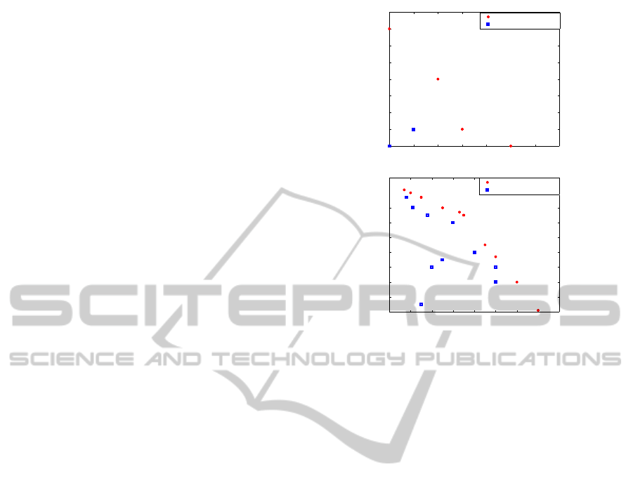
Example 1. We used the same example in (Dru-

gan and Nowe, 2013) because it simple to understand

and contains non-convex mean vector set. The num-

ber of arms |A| equals 6, the number of objectives D

equals 2. The standard deviation for arms in each

objective is 0.1. The true mean set vector is (µ

[0.55, 0.5]

, µ

= [0.53,0.51]

, µ

= [0.52,0.54]

= [0.5,0.57]

, µ

= [0.51,0.51]

, µ

= [0.5, 0.5]

Note that, the Pareto front is A

∗

= (a

∗

where a

∗

refers to the optimal arm i

∗

. The subopti-

mal a

is not dominated by the two optimal arms a

∗

and a

∗

, but a

∗

and a

∗

dominates a

while a

is domi-

nated by all the other mean vectors. Figure 3 shows a

set of 2-objective true mean with a non-convex set.

First, we compare the performance of the

SMOMAB and adaptive-SMOMAB algorithms. We

use either the standard algorithm, the adaptive algo-

rithm, or the genetic algorithm to set the weights.

Figure 4 gives the comparison of the SMOMAB and

adaptive-SMOMAB algorithms using the standard,

the adaptive, and the genetic algorithms. The stan-

dard deviation σ

i,r

of reward for each arm i in each

objective d is set to 0.1. The x-axis gives the time

step. The y-axis is the cumulative Pareto regret which

is the average of M experiments at each time step t.

Figure 4 shows that the SMOMAB algorithm per-

forms better than the adaptive-SMOMAB algorithm

using the adaptive, and the genetic algorithms, since

the cumulative Pareto regret is decreased. While, the

adaptive-SMOMAB algorithm performs slightly bet-

ter than the SMOMAB algorithm using the standard

algorithm.

Second, we compare the performance of the stan-

0.5 0.51 0.52 0.53 0.54 0.55 0.56 0.57

0.5

0.51

0.52

0.53

0.54

0.55

0.56

0.57

0.58

Objective

mean of optimal arm

mean of non optimal arm

0.49 0.5 0.51 0.52 0.53 0.54 0.55 0.56 0.57

0.49

0.5

0.51

0.52

0.53

0.54

0.55

0.56

0.57

0.58

Objective

mean of optimal arm

mean of non optimal arm

Figure 3: Non-convex and convex mean vector sets with

bi-objective. Upper ﬁgure shows a non-convex set with 6-

armed. Lower ﬁgure shows a convex set with 20-armed.

dard, the adaptive, and the genetic algorithms using

the adaptive-SMOMAB algorithm. Figure 5 gives the

cumulative Pareto regret. The x-axis is the time step.

The y-axis is the cumulative Pareto regret which is the

average of M experiments at each time step t. Figure 5

shows that the standard algorithm is the best algo-

rithm and the adaptivealgorithm is the worst one. The

mutation algorithm performs better than the adaptive

algorithm and slightly worse than the standard algo-

rithm.

In Example 1, the Pareto front A

∗

contains optimal

arms that are far from the non-optimal arms accord-

ing to the Euclidean distance and the number of the

optimal arms |A

∗

|, |A

∗

| = 4 is larger than the number

of the non-optimal arms which is equal 2. Therefore,

the SMOMAB algorithm almost performs better than

the adaptive-SMOMAB because it selects uniformly

at random one of the scalarized function. And, the

standard algorithm performs better than the adaptive

and the genetic algorithms because they generate new

weights that are nearest to each other to explore more

the optimal arms.

6.2 Triple-Objective

Example 2. With number of objectives D equals

2, number of arms |A| equals 20 and convex

Pareto mean set, (µ

= [.56,.491]

,µ

= [.55,

.51]

,µ

= [.54,.527]

,µ

= [.535, .535]

,µ

[.525, .555]

,µ

= [.523, .557]

,µ

= [.515, .56]

ICAART2015-InternationalConferenceonAgentsandArtificialIntelligence

0 50 100 150 200 250

5.4

5.6

5.8

6.2

6.4

6.6

6.8

x 10

−3

Time step

Cumulative Pareto Regret

adaptive−SMOMAB

SMOMAB

a. Using the standard algorithm

0 200 400 600 800 1000

x 10

−3

Time step

Cumulative Pareto Regret

adaptive−SMOMAB

SMOMAB

b. Using the adaptive algorithm

0 200 400 600 800 1000

x 10

−3

Time step

Cumulative Pareto Regret

adaptive−SMOMAB

SMOMAB

c. Using the genetic algorithm

Figure 4: Performance comparison of the SMOMAB

algorithm with the adaptive-SMOMAB algorithm on 2-

objective, 6-armed problem. The weights are set using the

standard algorithm in ﬁgure a, using the adaptive algorithm

in ﬁgure b, and using the genetic algorithm in ﬁgure c.

0 200 400 600 800 1000

x 10

−3

Time step

Cumulative Pareto Regret

Standard

Adaptive

Mutation

Figure 5: Performance comparison of the standard, the

adaptive, and the genetic algorithms on 2-objective, 6-

armed problem using the adaptive-SMOMAB algorithm.

0 200 400 600 800 1000

x 10

−3

Time step

Cumulative Pareto Regret

adaptive−SMOMAB

SMOMAB

a. Using the adaptive algorithm

Figure 6: Performance comparison of the SMOMAB

algorithm with the adaptive-SMOMAB algorithm on 3-

objective, 20-armed problem. The weights are set using the

adaptive algorithm.

= [.505,.567]

,µ

= [.5, .57]

,µ

= [.497,

.572]

,µ

= [.498,.567]

,µ

= [.501,.56]

,µ

[.505, .495]

,µ

= [.508, .555]

,µ

= [.51,.52]

= [.515,.525]

,µ

= [.52,.55]

,µ

[.53,.53]

,µ

= [.54,.52]

,µ

= [.54,.51]

the standard deviation for arms in each objective is

set to 0.1. The Pareto front A

∗

contains 10 optimal

arms, A

∗

= (a

∗

) (S.

Q. Yahyaa and Manderick, 2014c). Note that, the

number of the optimal arms |A

∗

|, |A

∗

| = 10 is equal

to the number of non-optimal arms and the optimal

arms are close to the non-optimal arm according

to the Euclidean distance. Figure 3 shows a set of

2-objective convex true mean vector set. We add

extra objective to Example 2, resulting in 3-objective,

20-armed bandit problem. The Pareto front A

∗

still

contains 10 optimal arms and the optimal arms are

closer to non-optimal arms compared to Example 2

according to the Euclidean distance.

First, we compare the performance of the

SMOMAB and adaptive-SMOMAB algorithms. We

use either the standard algorithm, the adaptive al-

gorithm, or the genetic algorithm to determine the

weight set. The adaptive-SMOMAB algorithm per-

forms better than the SMOMAB algorithm for the

standard, adaptive and genetic algorithms. Figure 6

gives the comparison of the SMOMAB and adaptive-

SMOMAB algorithms using the adaptive algorithm.

Figure 6 shows that the adaptive-SMOMAB algo-

rithm performs better than the SMOMAB algorithm

using the adaptive algorithm to set the weight set.

Second, we compare the performance of the stan-

dard, the adaptive, and the genetic algorithms using

the adaptive-SMOMAB algorithm. Figure 7 gives

the cumulative Pareto regret. Figure 7 shows that the

standard algorithm is the worst algorithm. The adap-

tive algorithm is the best one and performs slightly

better than the mutation algorithm. The mutation al-

ThompsonSamplingintheAdaptiveLinearScalarizedMultiObjectiveMultiArmedBandit

0 100 200 300 400 500

4.5

5.5

6.5

7.5

8.5

x 10

−3

Time step

Cumulative Pareto Regret

Standard

Adaptive

Mutation

Figure 7: Performance comparison of the standard, the

adaptive, and the genetic algorithms on 3-objective, 20-

armed problem using the adaptive-SMOMAB algorithm.

gorithm performs better than the standard algorithm

and worse than the adaptive algorithm.

From the above experiment, we see that when

we increase the number of objectives, the adaptive-

SMOMAB algorithm performs better than the

SMOMAB algorithm. Also, we see that the adap-

tive and the genetic algorithms perform better than the

standard algorithm.

6.3 5-Objective

We add extra 2 objectives to Example 2, resulting

in 5-objective, 20-armed bandit problem, leaving the

Pareto front A

∗

unchanged. The optimal arms in the

Pareto front A

∗

are still closer to the non-optimal arms

according to the Euclidean distance. The standard de-

viation for arms in each objective is set to 0.01.

First, we compare the performance of the

SMOMAB and adaptive-SMOMAB algorithms. We

use either the standard algorithm, the adaptive algo-

rithm, or the genetic algorithm to set the weights. The

adaptive-SMOMAB algorithm performs better than

the SMOMAB algorithm for all the weight setting.

Figure 8 gives the comparison of the SMOMAB and

adaptive-SMOMAB algorithms using the standard al-

gorithm. Figure 8 shows that the adaptive-SMOMAB

algorithm performs better than the SMOMAB algo-

rithm using the standard algorithm.

Second, we compare the performance of the stan-

dard, the adaptive, and the genetic algorithms using

the adaptive-SMOMAB algorithm. Figure 9 gives

the cumulative Pareto regret. Figure 9 shows that the

standard algorithm is the worst algorithm and the mu-

tation algorithm is the best algorithm. The adaptive

algorithm performs better than the standard algorithm

and worse than the mutation algorithm.

From the above experiment, we see that when we

increase the number of objectives, i.e. D > 3 the per-

formance of the adaptive-SMOMAB algorithm is in-

creased. We also see the performance of the genetic

0 200 400 600 800 1000

x 10

−3

Time step

Cumulative Pareto Regret

adaptive−SMOMAB

SMOMAB

a. Using the adaptive algorithm

Figure 8: Performance comparison of the SMOMAB

algorithm with the adaptive-SMOMAB algorithm on 5-

objective, 20-armed problem. The weights are set using the

adaptive algorithm.

0 200 400 600 800 1000

x 10

−3

Time step

Cumulative Pareto Regret

Standard

Adaptive

Mutation

Figure 9: Performance comparison of the standard, the

adaptive, and the genetic algorithms on 5-objective, 20-

armed problem using the adaptive-SMOMAB algorithm.

and adaptive algorithms are increased, where the cu-

mulative Pareto regret is decreased.

Discussion. from the above experiments, we see

that with minimum number of objectives D, D = 2,

the SMOMAB algorithm performs better than the

adaptive-SMOMAB algorithm. While, for number of

objectives D, D > 2 larger than 2, the performance

of the adaptive-SMOMAB algorithm is better than

the performance of the SMOMAB algorithm. As the

number of objectives is increased, the performance of

the adaptive-SMOMAB algorithm increases. We also

see that, for small number of objectives D, D = 2,

the standard algorithm performs better than the adap-

tive and the genetic algorithms using the adaptive-

SMOMAB algorithm. While as the number of ob-

jectives is increased, the adaptive and genetic algo-

rithms perform better than the standard algorithm us-

ing the adaptive-SMOMAB algorithm. Where, the

adaptive algorithm performs better than the genetic

algorithm for number of objectives equals 3 and the

genetic algorithm performs better than the adaptive

algorithm for number of objectives equals 5. The in-

tuition is that for small number of objectives D, D = 2

and small number of arms |A|, |A| = 6, the small num-

ICAART2015-InternationalConferenceonAgentsandArtificialIntelligence

ber of scalarized functions S, |S| = D+ 1 was able to

identify almost all the optimal arm in the Pareto front

∗

. While, for large number of objectives D, D ≥ 2

and large number of arms |A|, |A| = 20, the adaptive

and genetic algorithms generate new weights, and the

new weights explore all the optimal arms in the Pareto

front A

∗

. We also see that the ﬁgures have a ﬂat per-

formance and this is because of the calculation of the

Pareto regret. Pareto regret adds minimum distance

(virtual distance) to the selected suboptimal arm to

create an optimal arm, therefore the added distance

will be the same if the suboptimal arms are close to

each other.

7 CONCLUSIONS

We presented multi-objective, multi-armed bandit

(MOMAB) problem and the regret measures in the

MOMAB. We presented the linear scalarized function

and the linear scalarized-KG that transform the multi-

objective problem into a single problem by summing

the weighted objectivesto ﬁnd the optimal arms. Usu-

ally, the scalarized multi-objective (SMOMAB) algo-

rithm selects uniformly at random the scalarized func-

tion s. We proposed to use techniques from the multi-

objective optimization in the SMOMAB algorithm to

adapt the weights online. We use the genetic opera-

tors to generate new weights in the proximity of the

current weight sets, and we adapt the weights to be

perpendicular on the set of Pareto optimal solutions.

We propose the adaptive scalarized multi-armed ban-

dit (adaptive-SMOMAB) algorithm that uses Thomp-

son sampling policy to select the scalarized s. We

experimentally compared the SMOMAB algorithm

and the adaptive-SMOMAB algorithm using the pro-

posed algorithms: the ﬁxed weights, the adaptive

weights, and the genetic weights. We conclude that

when the number of objective D is increased D >

2, the adaptive-SMOMAB performs better than the

SMOMAB algorithm. The adaptive and the mutation

algorithms perform better than the standard algorithm

(ﬁxed weights).

REFERENCES

Das, I. and Dennis, J. E. (1997). A closer look at drawbacks

of minimizing weighted sums of objectives for pareto

set generation in multicriteria optimization problems.

Structural Optimization, 14(1):63–69.

Drugan, M. (2013). Sets of interacting scalarization func-

tions in local search for multi-objective combinatorial

optimization problems. In IEEE Symposium Series on

Computational Intelligence (IEEE SSCI).

Drugan, M. and Nowe, A. (2013). Designing multi-

objective multi-armed bandits algorithms: A study. In

Proceedings of the International Joint Conference on

Neural Networks (IJCNN).

Drugan, M. and Thierens, D. (2010). Geometrical recombi-

nation operators for real-coded evolutionary mcmcs.

Evolutionary Computation, 18(2):157–198.

Eichfelder, G. (2008). Adaptive Scalarization Methods in

Multiobjective Optimization. Springer-Verlag Berlin

Heidelberg, 1st edition.

I. O. Ryzhov, W. P. and Frazier, P. (2011). The knowledge-

gradient policy for a general class of online learning

problems. Operation Research.

J. Dubois-Lacoste, M. L.-I. and Stutzle, T. (2011). Improv-

ing the anytime behavior of two-phase local search. In

Annals of Mathematics and Artiﬁcial Intelligence.

Powell, W. B. (2007). Approximate Dynamic Program-

ming: Solving the Curses of Dimensionality. John

Wiley and Sons, New York, USA, 1st edition.

S. Q. Yahyaa, M. D. and Manderick, B. (2014a). Empir-

ical exploration vs exploitation study in the scalar-

ized multi-objective multi-armed bandit problem. In

International Joint Conference on Neural Networks

(IJCNN).

S. Q. Yahyaa, M. D. and Manderick, B. (2014b). Knowl-

edge gradient for multi-objective multi-armed bandit

algorithms. In International Conference on Agents

and Artiﬁcial Intelligence (ICAART), France. Inter-

national Conference on Agents and Artiﬁcial Intelli-

gence (ICAART).

S. Q. Yahyaa, M. D. and Manderick, B. (2014c). Multi-

variate normal distribution based multi-armed bandits

pareto algorithm. In the European Conference on Ma-

chine Learning and Principles and Practice of Knowl-

edge Discovery in Databases (ECML/PKDD).

Thompson, W. R. (1933). On the likelihood that one un-

known probability exceeds another in view of the evi-

dence of two samples. In Biometrika.

Zitzler, E. and et al. (2002). Performance assessment

of multiobjective optimizers: An analysis and re-

view. IEEE Transactions on Evolutionary Computa-

tion, 7:117–132.

ThompsonSamplingintheAdaptiveLinearScalarizedMultiObjectiveMultiArmedBandit