Plane Fitting and Depth Variance Based Upsampling for Noisy Depth

Map from 3D-ToF Cameras in Real-time

Kazuki Matsumoto, Francois de Sorbier and Hideo Saito

Graduate School of Science and Technology, Keio University, 3-14-1 Hiyoshi, Kohoku-ku, Yokohama, Kanagawa, Japan

Keywords:

Depth map, ToF depth sensor, GPU, Plane Fitting, Upsampling, denoising.

Abstract:

Recent advances of ToF depth sensor devices enables us to easily retrieve scene depth data with high frame

rates. However, the resolution of the depth map captured from these devices is much lower than that of color

images and the depth data suffers from the optical noise effects. In this paper, we propose an efﬁcient algorithm

that upsamples depth map captured by ToF depth cameras and reduces noise. The upsampling is carried out

by applying plane based interpolation to the groups of points similar to planar structures and depth variance

based joint bilateral upsampling to curved or bumpy surface points. For dividing the depth map into piecewise

planar areas, we apply superpixel segmentation and graph component labeling. In order to distinguish planar

areas and curved areas, we evaluate the reliability of detected plane structures. Compared with other state-of-

the-art algorithms, our method is observed to produce an upsampled depth map that is smoothed and closer to

the ground truth depth map both visually and numerically. Since the algorithm is parallelizable, it can work in

real-time by utilizing highly parallel processing capabilities of modern commodity GPUs.

1 INTRODUCTION

In recent years, depth images have gained popularity

among many research ﬁelds including 3D reconstruc-

tion for dynamic scenes, augmented reality and en-

vironment perception in robotics. Depth images are

often obtained by stereo vision techniques, which are

computationally expensive and not able to calculate

the range data in non-texture scenes. This problem

was solved by the development of 3D time-of-ﬂight

(3D-ToF) depth cameras, such as MESA Swissranger

and SoftKinetic DepthSense. A light source from the

camera emits a near-infrared wave to 3D objects and

the reﬂected light from scene objects is captured by

a dedicated sensor. By calculating the phase shift be-

tween the emitted light and the received one, the dis-

tance at each pixel can be estimated. Thus, ToF depth

cameras can acquire the range data even from texture-

less scenes in high frame rates.

However, the depth map captured by ToF depth

camera is unable to satisfy the requirements for de-

veloping rigorous 3D applications. This is due to the

fact that the resolution of the depth image is relatively

low (e.g. 160 × 120 pixels for SoftKinetic Depth-

Sense DS311) and the data is heavily contaminated

with structural noise. Moreover, the noise increases if

the infrared light interferes with other light sources or

is reﬂected irregularly by the objects.

In this paper, we propose joint upsampling and

denoising algorithm for depth data from ToF depth

cameras, which is based on local distribution of the

depth map. The upsampling is performed by simulta-

neously exploiting the depth variance based joint bi-

lateral upsampling and the plane ﬁtting based on the

locally planar structures of the depth map. In order to

detect the planar area, we combine normal-adaptive

superpixel segmentation and graph component label-

ing. Our algorithm can discriminate between planar

surfaces and curved surfaces based on the reliability

of estimated local planar surface structure. Therefore

we can apply plane ﬁtting to truly planar distributed

areas and utilize depth variance based joint bilateral

upsampling to curved or bumpy areas. As a result,

we can generate a smooth depth map while preserv-

ing curved surfaces. By using massively parallel com-

puting capabilities of modern commodity GPUs, the

method is able to maintain high frame rates. The re-

mainder of this paper is structured as follows. In Sec-

tion 2, we will discuss related works. After describing

the overview and the details of our technique in Sec-

tion 3. Section 4 will show the result of experiments

and discuss them. Finally we will conclude the paper

in Section 5.

150

Matsumoto K., de Sorbier F. and Saito H..

Plane Fitting and Depth Variance Based Upsampling for Noisy Depth Map from 3D-ToF Cameras in Real-time.

DOI: 10.5220/0005184801500157

In Proceedings of the International Conference on Pattern Recognition Applications and Methods (ICPRAM-2015), pages 150-157

ISBN: 978-989-758-077-2

 2015 SCITEPRESS (Science and Technology Publications, Lda.)

2 RELATED WORKS

In order to upsample the depth data captured by a

ToF depth camera, several approaches have been pro-

posed which can be divided into two groups. The ﬁrst

one deals with the instability of depth data provided

by the RGB-D camera by using several depth images

for reducing variations over each pixel depth value

(Camplani and Salgado, 2012) (Dolson et al., 2010).

However, these methods can not cope with numerous

movement of objects in captured scenes or require the

camera to be stationary.

The second group applies upsampling methods on

only one pair of depth and color images for inter-

polating depth data while reducing structural noise.

Among these methods, Joint Bilateral Upsampling

(Kopf et al., 2007) and the interpolation method

based on the optimization of a Markov Random Field

(Diebel and Thrun, 2005) are the most popular ap-

proaches. They exploit information from RGB im-

ages to improve the resolution of depth data under the

assumption that depth discontinuities are often related

to color changes in the corresponding regions in the

color image. However the depth data captured around

object boundaries is not reliable and heavily contam-

inated with noise.

(Chan et al., 2008) solved this problem by intro-

ducing a noise-aware bilateral ﬁlter, which blends the

results of standard upsampling and joint bilateral ﬁl-

tering depending on the depth map’s regional struc-

ture. The drawback of this method is it can some-

times smooth the ﬁne details of depth maps. (Park

et al., 2011) proposed a high quality depth map up-

sampling method. Since it extends nonlocal means

ﬁltering with an additional edge weighting scheme, it

requires a lot of computational time.

(Matsuo and Aoki, 2013) presented a depth im-

age interpolation method by estimating tangent planes

based on superpixel segmentation. In this method,

depth interpolation is achieved within each region by

using Joint Bilateral Upsampling. (Soh et al., 2012)

also use superpixel segmentation for detecting piece-

wise planar surfaces. In order to upsample the low-

resolution depth data, they apply plane based interpo-

lation and Markov Random Field based optimization

to locally detected planar areas. These approaches can

adapt the processing according to local object shapes

based on the information form each segmented re-

gion.

Inspired from these approaches, we also use su-

perpixel segmentation for detecting locally planar

surfaces and exploit the structure of detected areas.

Compared with other superpixel based methods, our

method can relatively smooth depth map in real-time.

3 PROPOSED METHOD

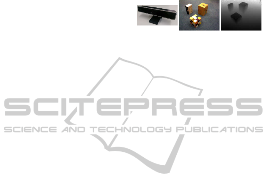
Figure 1: Left: SoftKinetic DepthSense DS311. Center:

captured color image. Right: captured depth image.

As Figure 1 shows, we use SoftKinetic DepthSense

DS311 for our system, which can capture 640 × 480

color images and 160 × 120 depth maps at 25-60fps.

Before applying our method, we project each 3D

data from depth map onto its corresponding color im-

age by using rigid transformation obtained from cam-

era calibration between color camera and depth sen-

sor. In our experiment, we use the extrinsic parame-

ters given from a DepthSense DS311. After this pro-

cess, we can obtain RGB-D data in color image coor-

dinate frame.

However, it is still low resolution and includes

much noise and occluded depth data around the ob-

ject boundaries due to slight differences depth cam-

era and color camera positions. Therefore, we ﬁrst

apply depth variance based joint bilateral upsampling

to the RGB-D data and generate highly smoothed and

interpolated depth map. Next, we calculate the nor-

mal map by applying the method proposed by (Holzer

et al., 2012). By using this normal map, we apply

normal-adaptivesuperpixel segmentation for dividing

the 3D depth map into clusters so that the 3D points in

each cluster make up a planar structure. For merging

clusters which are located on the same plane, graph

component labeling is utilized to segment image by

comparing the normals of each cluster. The plane

equation of each cluster is computed from the nor-

mal and center point associated with the cluster. After

that, we evaluate the reliability of each plane and dis-

criminate between planar cluster and curved cluster

and apply plane ﬁtting and optimization to the depth

map. As a result, our method can generate smooth

depth maps which still contain complex shape infor-

mation.

3.1 Depth Variance Based Joint

Bilateral Upsampling

Joint Bilateral Upsampling(JBU) is a modiﬁcation of

the bilateral ﬁlter, an edge-preserving smoothing ﬁlter

for intensity images. The smoothed depth value D

at the pixel p is computed from its neighboring pixels

PlaneFittingandDepthVarianceBasedUpsamplingforNoisyDepthMapfrom3D-ToFCamerasinReal-time

151

Ω as follows:

∑

q∈Ω

(p− q)g

−C

− D

∑

q∈Ω

(p− q)g

−C

− D

)

(1)

where g

, g

are Gaussian functions controlled by

the standard deviation parameters σ

Cσ

respec-

tively. p − q represents the spatial distance, C

− C

is color similarity and D

− D

is the depth similarity.

As this equation shows, JBU locally shapes the spatial

smoothing kernel by multiplying it with a color simi-

larity term and a range term, and thus the edges can be

preserved while the non-edge regions are smoothed.

However, the depth map obtained from ToF depth

camera includes so much noise around the object

boundaries that JBU can suffer from the effects of the

noise. In order to remove the noise, we ﬁrst calculate

the mean and standard deviation of speciﬁed depth

value around each pixel and if the variance is over the

threshold, the depth data is removed. After that, the

standard deviation is modiﬁed according to the depth

error’s quadratic dependance of distance deﬁned by

(Anderson et al., 2005) as follows:

′

cos(θ)σ

(2)

where σ

′

, D

and θ are the local standard deviation,

the local mean and the angle of incidence of infrared

light. Then, σ

is adapted to better reduce the noise

and preserve the edges as follows:

= max{σ

+ λ· σ

′

,σ

min

} (3)

where σ

is a relatively high sigma of g

, σ

min

is the

minimum value, and λ is a negative factor. This mod-

iﬁcation is based on (Chen et al., 2012). Figure 2

shows the depth map captured in the scene of Figure

1 and the depth maps upsampled by JBU and depth

variance based JBU. Compared with the center image,

the noise around the object boundaries is removedand

the depth map is properly upsampled in right image.

After applying this technique, the smoothed and up-

sampled depth map is projected into 3D coordinates

using the intrinsic parameters of the color camera.

Figure 2: Left: input depth map. Center: JBU. Right: depth

variance based JBU.

3.2 Normal Estimation

After utilizing joint bilateral upsampling, the normal

estimation technique (Holzer et al., 2012) is applied

to the 3D points for computing a normal map in real-

time. This technique can generate a smooth normal

map by employing an adaptive window size to ana-

lyze local surfaces. As this approach also uses integral

images for reducing computational cost and can be

implemented in GPU, we can calculate normal maps

at over 50fps. However, this method can’t estimate

normals in the pixels around the object boundaries.

Therefore, we interpolate the normal map by calculat-

ing the outer product of two close points around these

invalid pixel vertices. The estimated normal map is

visualized in Figure 3.

3.3 Normal Adaptive Superpixel

Segmentation

(Weikersdorfer et al., 2012) proposed a novel over-

segmentation technique, Depth-adaptive superpixels

(DASP), for RGB-D images so that the 3D geom-

etry surface is partitioned into uniformly distributed

and equally sized planar patches. This clustering al-

gorithm assigns points to superpixels and improves

their centers using iterative k-means algorithms with

a distance computed from not only color distance and

spatial distance but also the depth value and normal

vector. By using the color image, the depth map cal-

culated in Section 3.1 and the normal map generated

in Section 3.2, we modify the DASP to use gSLIC

method by (Ren and Reid, 2011) in GPU.

The distance dist

) between cluster k and a

point p

is calculated as follows:

dist

) =

∑

dist

)

∑

(4)

with the subscript j consecutively representing the

spatial(s), color(c), depth(d) and normal(n) terms. w

, w

and w

are empirically deﬁned weights of

spatial, color, depth and normal distances, respec-

tively represented as dist

), dist

)

and dist

). Figure 3 illustrates the result of normal

adaptive superpixels, where the scene is segmented as

each region is homogeneous in terms of color, depth

and normal vector. The normal adaptive superpixel

segmentation gives for each cluster its C

)

and its representative normal n

(a,b,c). As a result,

each point V

) located on a locally pla-

nar surface of a cluster k can be represented as follows

+ bY

+ cZ

= d

(5)

where d

is the distance between the plane and the ori-

gin. Assuming thatC

is located on the planar surface,

we can calculate d

as follows.

= aX

+ bY

+ cZ

(6)

ICPRAM2015-InternationalConferenceonPatternRecognitionApplicationsandMethods

152

Figure 3: RGB image: normal image: normal adaptive superpixels: merging superpixels.

3.4 Merging Superpixels

Since the superpixel segmentation is over-

segmentation proceduce, the post-processing is

required to ﬁnd global planar structures. (Weikers-

dorfer et al., 2012) also provides the spectral grapth

theory, which extracts global shape information

from local pixel similarity. However, it requires

much computational time because it is not a parallel

procedure and can not be implemented in GPU.

Therefore, we apply graph component labeling with

GPUs and CUDA proposed by (Hawick et al., 2010)

to segmented images as illustrated in Algorithm 1.

By considering each representative planar equation

in given superpixel’s clusters, the labeling process is

carried out for merging clusters which are distributed

on the same planar area.

As Figure 3 shows, we can obtain the global pla-

nar area while preserving small planar patches in real-

time. Finally, the center and the representativenormal

vector of each region are computed again by taking

the average of normals and center points of the super-

pixels in each region.

3.5 Plane Fitting and Optimization

By using equation (5), 3D coordinates

) on planar cluster k are com-

puted from normalized image coordinates u

)

as follows:

+ by

+ c

= x

= y

(7)

By judging from the reliability of the plane model cal-

culated during the previous step, we can detect which

clusters are planar. The optimized point V

is gener-

ated by using V

computed from the depth variance

based JBU in section 3.1 and the variance of normal

vectors ψ

obtained in section 3.4 as follows:







(|V

−V

| > γ

cos(θ)

or ψ

> δ)

cosψ

(1.0− cosψ

) (otherwise)

(8)

Algorithm 1: Superpixel Merging Algorithm.

function LabelEquivalenceHost(D,Size)

declare integer L[Size], R[Size]

do in parallel initialize L[0...Size − 1] and

R[0...Size−1] such that L[i] ← NASP[i] and R[i] ← i

declare boolean m

repeat

do in parallel in all pixels call

Scanning(D, L,R,m) and Labeling(D,L,R)

until m = false

return

function Scanning(D, L,R,m)

declare integer id,label

,label

[9]

id ←pixel ithread ID)

label

,label

← L[id]

←neighbors of id

for all id

∈ q

declare ﬂoat d

,θ

← |d

NASP[id]

− d

NASP[id

]

← arccos(n

NASP[id]

× n

NASP[id

]

)

if d

< α and θ

< β then

min(label

,L[id

])

end if

end for

if label

< label

then

atomicMin(R[label

],label

)

m ← true

end if

return

function Labeling(D, L,R)

declare integer id,ref

id ←pixel (thread ID)

if L[id] = id then

ref ← R[id]

repeat

ref ← R[ref]

until ref = R[ref]

R[ref] ← ref

end if

L[id] ← R[L[id]]

return

PlaneFittingandDepthVarianceBasedUpsamplingforNoisyDepthMapfrom3D-ToFCamerasinReal-time

153

where θ is the incident angle of the infrared light from

a depth camera, γ and δ are the adaptively changing

thresholds speciﬁcally chosen for a given scene for

rejecting unreliable plane models. The huge error of

plane ﬁtting will be removed by setting the threshold

γ. The threshold δ can prevent plane ﬁtting from be-

ing applied to curved surfaces. Finally, we apply or-

dinary bilateral ﬁlter to V

for smoothing the artifacts

around boundaries.

4 EXPERIMENTS

We applied our method on two different scenes

captured by SoftKinetic DepthSense DS311(color:

640 × 480, depth: 160 × 120) and compared our re-

sult(PROPOSED) with other related works, Joint

Bilateral Filtering based Upsampling(JBF), Markov

Random Field(MRF), DISSS proposed by (Matsuo

and Aoki, 2013) and SPSR presented by (Soh et al.,

2012) in terms of runtime and qualitative evalua-

tion. For the quantitative evaluation, we gener-

ated the ground truth depth data with a scene ren-

dered via OpenGL. The ground truth depth data was

downsampled and added noise according to the noise

model of ToF depth camera described in (Anderson

et al., 2005). Then, we applied all methods to the

noisy depth data and calculated root-mean-square-

error(RMSE) and peak signal-to-noise ratio(PSNR)

between ground truth and the results in order to com-

pare the accuracy of all the methods. All processes

are implemented on a PC with Intel Core i7-4770K,

NVIDIA GeForce GTX 780, and 16.0GB of mem-

ory. We used OpenCV for trivial visualizations of

color and depth images as well as data manipulations,

and PointCloudLibrary for 3-dimensional visualiza-

tion. All GPGPU implementations were done using

CUDA version 5.0.

4.1 Qualitative Evaluation

Table 1 shows the parameters for each experiment.

We adjust the parameters for the superpixel segmen-

tation and merging superpixels so that we can divide

the depth map into truly planar areas. As Figure 6 and

7 demonstrate, our technique can generate smooth

and high resolution depth maps form low resolution

and noisy data captured by ToF depth camera. MRF

and JBF suffer from noisy data since these methods

estimate a pixel depth value from its neighborhood.

DISSS also applies joint bilateral upsampling in esti-

mated homogeneous surface regions and can’t repro-

duce smooth depth map. The upsampled depth map

from SPSR is smoothed because it uses both plane ﬁt-

ting and markov random ﬁeld to upsample the depth

data based on local planar surface equation estimated

by superpixel segmentation. However, as Figure 10

shows, ﬁssures appear around the boundaries of each

region in the upsampled depth map because the su-

perpixel segmentation is processed locally. Figure 10

also shows that our method can obtain denoised depth

map particularly in areas of planar surfaces while pre-

serving the curved surfaces and the detail of objects

with complex shapes (e.g. the depth map of stanford

bunny). The reason is that our method can ﬁnd global

planar areas and adapt the upsampling method based

on detected surface structures. Thanks to the prepro-

cessing explained in section 3.1, we can remove the

noise around the object boudaries as shown in Fig-

ure 9. In order to compare the runtime, all the meth-

ods are implemented with GPU and each runtime is

shown in Figure 4. Compared with other superpixel

based methods, our technique requires far less com-

putational time as shown in Figure 4.

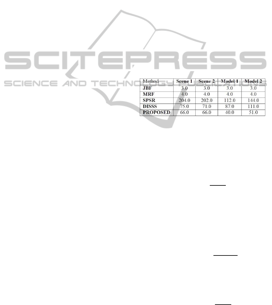
Figure 4: Runtime (msec).

4.2 Quantitative Evaluation

Based on the characterization of the ﬂash ladar de-

vices (Anderson et al., 2005), we presumed that the

depth value variance σ(p,d

) at pixel p is discribed

as follows:

σ(p,d

) = k

cos(θ)

(9)

where d

is the depth value acquired from ground

truth depth data, θ is the incident angle of the infrared

light from a depth camera and k is the noise coefﬁ-

cient. By using Box-Muller transform and equation

9, we added normally distributed random noise to the

downsampled ground truth depth based on the proba-

bility distribution described as follows:

p(d|d

, p) ∝ exp



−

(d − d

)

σ(p,d

)



(10)

In order to evaluate the effectiveness of all meth-

ods, we applied them to noisy downsampled depth

data (640× 480,320× 240, 160× 120)and calculated

RMSE and PSNR. PSNR can be written as follows:

PSNR = 20log



max

RMSE



(11)

ICPRAM2015-InternationalConferenceonPatternRecognitionApplicationsandMethods

154

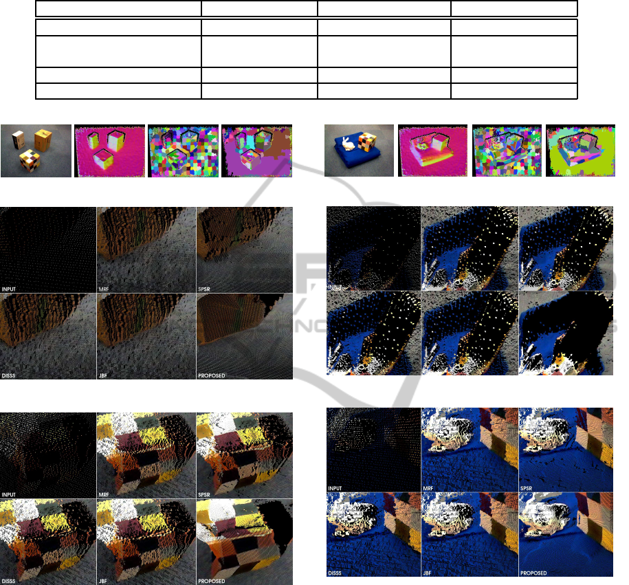
Table 1: Parameters for experiment.

Method Parameters Scene 1 Scene 2

Depth Variance Based JBU σ

, σ

, λ, σ

min

30, 50 , 100, −10, 15 70, 50 , 20, −10, 15

Superpixel Segmentation w

, w

50, 50 , 50, 150 50, 50 , 50, 150

iteration, clusters 1, 300 1, 300

Merging Superpixels@ α, β 220mm, π/8 75mm, π/12

Optimization@ γ, δ 0.0001, π/8 0.0001, π/8

Figure 5: RGB: normals: superpixels: merging superpixels.

Figure 6: Scene 1(a).

Figure 7: Scene 1(b).

Model 1 consists of three planar surfaces and Fig-

ure 11 shows the result of the experiment with Model

1. Our technique can generate the closest depth map

to the ground truth depth data because the method re-

places the noisy depth map entirely with a plane ﬁtted

depth map. Model 2 is composed of planar surfaces

and curved surfaces. As Figure 13 illustrates, pro-

posed method is the most accurate method and SPSR

is the second of all the methods. Since SPSR applies

the plane ﬁtting and MRF optimization to local pla-

nar patches, the noise reduction is performed locally

and that sometimes leads to ﬁssure like discontinu-

ities around the edges of each region as we discussed

Figure 8: RGB: normals: superpixels: merging superpixels.

Figure 9: Scene 2(a).

Figure 10: Scene 2(b).

in 4.1. Moreover, the runtime of SPSR is the slowest

of all methods because of the edge reﬁnement of su-

perpixel boundaries as shown in Table 4. Our method

is slower than JBF and MRF but it can still main-

tain high frame rates because of parallel processing

implemented in GPU. Our technique can reproduce

relatively accurate depth map compared with other

methods because it can distinguish planar regions and

curved regions and apply the appropriate algorithms

by combining planar ﬁtting and depth variance based

joint bilateral upsampling. To conclude, our tech-

nique clearly outperforms other methods, in terms of

runtime, visual assessment and accuracy.

PlaneFittingandDepthVarianceBasedUpsamplingforNoisyDepthMapfrom3D-ToFCamerasinReal-time

155

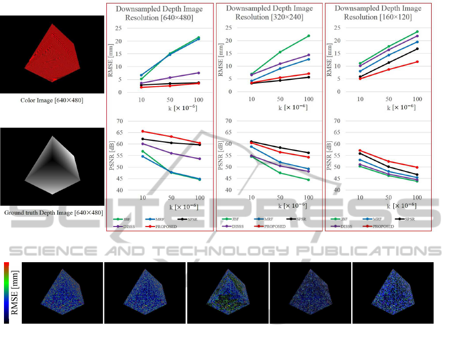
Figure 11: Model 1 RMSE and PSNR (d

max

= 3622.93mm).

JBF MRF

SPSR

DISSS

PROPOSED

Figure 12: Model 1 Visualization of RMSE (Input depth isize[160× 120], k=50×10

−6

5 CONCLUSIONS

In this work, we proposed a depth image upsampling

and denoising algorithm, which has a low resolution

depth image from ToF depth camera and a high reso-

lution color image as its inputs. In order to detect pla-

nar structures,we combined normal adaptive super-

pixels and graph component labeling by simultane-

ously using color image, depth data and normal map.

As our method can properly apply plane ﬁtting and

depth variance based joint bilateral ﬁlter according to

the local points structure, it can generate smoothed

depth map retaining the shape of curved surfaces.

Our experimental results show that this technique

can upsample depth images more accurately than pre-

vious methods, particularly when applied to a scene

with large planar areas. Since the algorithm is paral-

lelizable, our framework can achieve real-time frame

rates thanks to GPGPU acceleration via CUDA archi-

tecture, which becomes crucial when such a method is

used in computationally expensive applications, such

as 3D reconstruction and SLAM.

ACKNOWLEDGEMENTS

This work is partially supported by National Insti-

tute of Information and Communications Technology

(NICT), Japan.

REFERENCES

Anderson, D., Herman, H., and Kelly, A. (2005). Experi-

mental characterization of commercial ﬂash ladar de-

vices. In International Conference of Sensing and

Technology, volume 2.

Camplani, M. and Salgado, L. (2012). Adaptive spatio-

temporal ﬁlter for low-cost camera depth maps. In

Emerging Signal Processing Applications (ESPA),

2012 IEEE International Conference on, pages 33–36.

IEEE.

Chan, D., Buisman, H., Theobalt, C., Thrun, S., et al.

(2008). A noise-aware ﬁlter for real-time depth up-

sampling. In Workshop on Multi-camera and Multi-

modal Sensor Fusion Algorithms and Applications-

M2SFA2 2008.

ICPRAM2015-InternationalConferenceonPatternRecognitionApplicationsandMethods

156

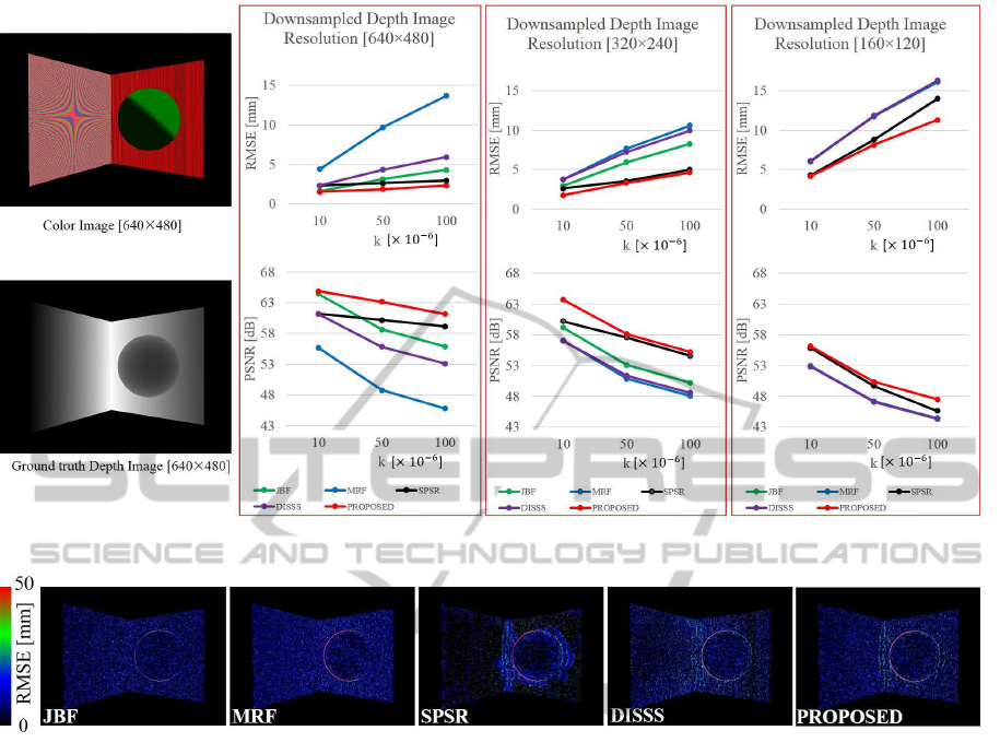
Figure 13: Model 2 RMSE and PSNR (d

max

= 2678.52mm).

Figure 14: Model 2 Visualization of RMSE (Input depth size [320× 240], k=50 ×10

−6

Chen, L., Lin, H., and Li, S. (2012). Depth image enhance-

ment for kinect using region growing and bilateral ﬁl-

ter. In Pattern Recognition (ICPR), 2012 21st Inter-

national Conference on, pages 3070–3073. IEEE.

Diebel, J. and Thrun, S. (2005). An application of markov

random ﬁelds to range sensing. In Advances in neural

information processing systems, pages 291–298.

Dolson, J., Baek, J., Plagemann, C., and Thrun, S. (2010).

Upsampling range data in dynamic environments. In

Computer Vision and Pattern Recognition (CVPR),

2010 IEEE Conference on, pages 1141–1148. IEEE.

Hawick, K. A., Leist, A., and Playne, D. P. (2010). Par-

allel graph component labelling with gpus and cuda.

Parallel Computing, 36(12):655–678.

Holzer, S., Rusu, R. B., Dixon, M., Gedikli, S., and Navab,

N. (2012). Adaptive neighborhood selection for real-

time surface normal estimation from organized point

cloud data using integral images. In Intelligent Robots

and Systems (IROS), 2012 IEEE/RSJ International

Conference on, pages 2684–2689. IEEE.

Kopf, J., Cohen, M. F., Lischinski, D., and Uyttendaele, M.

(2007). Joint bilateral upsampling. In ACM Transac-

tions on Graphics (TOG), volume 26, page 96. ACM.

Matsuo, K. and Aoki, Y. (2013). Depth interpolation

via smooth surface segmentation using tangent planes

based on the superpixels of a color image. In Com-

puter Vision Workshops (ICCVW), 2013 IEEE Inter-

national Conference on, pages 29–36. IEEE.

Park, J., Kim, H., Tai, Y.-W., Brown, M. S., and Kweon, I.

(2011). High quality depth map upsampling for 3d-tof

cameras. In Computer Vision (ICCV), 2011 IEEE In-

ternational Conference on, pages 1623–1630. IEEE.

Ren, C. Y. and Reid, I. (2011). gslic: a real-time imple-

mentation of slic superpixel segmentation. University

of Oxford, Department of Engineering, Technical Re-

port.

Soh, Y., Sim, J.-Y., Kim, C.-S., and Lee, S.-U. (2012).

Superpixel-based depth image super-resolution. In

IS&T/SPIE Electronic Imaging, pages 82900D–

82900D. International Society for Optics and Photon-

ics.

Weikersdorfer, D., Gossow, D., and Beetz, M. (2012).

Depth-adaptive superpixels. In Pattern Recognition

(ICPR), 2012 21st International Conference on, pages

2087–2090. IEEE.

PlaneFittingandDepthVarianceBasedUpsamplingforNoisyDepthMapfrom3D-ToFCamerasinReal-time

157