
HyperSAX: Fast Approximate Search of Multidimensional Data
Jens Emil Gydesen, Henrik Haxholm, Niels Sonnich Poulsen, Sebeastian Wahl and Bo Thiesson
Department of Computer Science, Aalborg University, Aalborg Øst, Denmark
Keywords:
Data Mining, Indexing, Approximate Search, Multidimensional Data, Images, Data Representation.
Abstract:
The increasing amount and size of data makes indexing and searching more difficult. It is especially chal-
lenging for multidimensional data such as images, videos, etc. In this paper we introduce a new indexable
symbolic data representation that allows us to efficiently index and retrieve from a large amount of data that
may appear in multiple dimensions. We use an approximate lower bounding distance measure to compute the
distance between multidimensional arrays, which allows us to perform fast similarity searches. We present
two search methods, exact and approximate, which can quickly retrieve data using our representation. Our ap-
proach is very general and works for many types of multidimensional data, including different types of image
representations. Even for millions of multidimensional arrays, the approximate search will find a result in a
few milliseconds, and will in many cases return a result similar to the best match.
1 INTRODUCTION
The increasing amount of data we collect, create, and
generate necessitate new and better ways of indexing
and searching. It is especially true for multidimen-
sional data. Multidimensional data may appear as im-
ages, videos, multidimensional geometric objects or
something completely different. In many applications
we often want to search and compare data to other
data, which can be expensive in terms of I/O opera-
tions and computations. An example of an applica-
tion using search and comparison is image searching,
i.e. searching using an image as the query, which is
provided by, for instance, the image search engines
from Google, Bing, and TinEye. Smart indexing tech-
niques decrease the amount of I/O operations and can
provide very fast index searching.
Data often involves an encoding of a spatial or
temporal structure. An example would be time se-
ries, i.e. measurements over time. For the purpose
of this paper, we will look at time series as one-
dimensional arrays (i.e. a fixed-length indexed se-
quences of numbers starting at index 0) represented
by a function f (t) = v, with a v value for each t (time)
value. We can extend this definition to accommodate
multidimensional data structured as multidimensional
arrays. For an array of n dimensions, we can define
the function f (t) = v, where t is an n-tuple of integers
(t
1
,...,t
n
) that map to a single v value. We also de-
fine the size of a multidimensional array as an n-tuple
m = (m
1
,...,m
n
), where 0 ≤ t
i
< m
i
for 1 ≤ i < n.
For convenience purposes, we will use the notation of
A
t
1
,...,t
n
to denote multidimensional array access, in-
stead of f (t). Images will by used as examples of
multidimensional data, but we emphasize that our ap-
proach also generalizes to other types of multidimen-
sional data. Consider an 8-bit gray scale image (2-
dimensional). Here each pixel (x,y) within the image
will map to a single v value between 0 and 255. While
it is possible to imagine that v could also be a tuple or
a vector (such as R, G and B values for color images),
we will only consider v as a single value (see Sec-
tion 1.1 for our representation of color images).
We can generalize this structure to an arbitrary
number of dimensions, and given our similar defi-
nitions of time series and multidimensional arrays,
we can base our approach on indexing techniques for
time series, such as iSAX (Shieh and Keogh, 2008)
(described in Section 2).
Several search methods and data structures to in-
dex time series have been proposed (Andr
´
e-J
¨
onsson,
2002; Keogh et al., 2001b; Faloutsos et al., 1994), but
only few efficient methods exist for multidimensional
arrays. Gaede and G
¨
unther (1998) have collected and
compared some methods for accessing and indexing
multidimensional data, using point access methods
or spatial access methods. Here they compare some
spatial tree data structures (among others) such as R-
tree and its variants, quadtree, k-d tree, KDB-tree and
buddy tree.
190
Gydesen J., Haxholm H., Poulsen N., Wahl S. and Thiesson B..
HyperSAX: Fast Approximate Search of Multidimensional Data.
DOI: 10.5220/0005185201900198
In Proceedings of the International Conference on Pattern Recognition Applications and Methods (ICPRAM-2015), pages 190-198
ISBN: 978-989-758-076-5
Copyright
c
2015 SCITEPRESS (Science and Technology Publications, Lda.)

In this paper we introduce a new symbolic rep-
resentation called hyperSAX which can be used to
index multidimensional data. The difference be-
tween our approach and these multidimensional in-
dexing techniques is that we discretize and quantize
the data, much like iSAX. The difference between
our approach and iSAX is, of course, that we index
multidimensional data, rather than time series, and
that we split on both the structure of the data and
the values. Furthermore our representation allows
for dynamic word lengths instead of predefined static
word lengths. A definition of word length and the
more general notation of a split can be found in Sec-
tion 2. With our hyperSAX representation we can de-
fine lower bounding approximate distance measures
to compare multidimensional arrays very fast, and we
will thus be able to perform very fast searching.
1.1 Image Indexing
Images can be indexed based on different features,
such as colors, shapes, size, texture or objects inside
the image. We will in this paper, as an example, index
images based on their colors, but our approach will
work using other types of features. We have already
mentioned how data for a gray scale image would be
structured. We add another dimension for colored im-
ages representing the color channels. If we, for ex-
ample, have a 24-bit RGB image, the input tuple t
would consist of an x-coordinate, a y-coordinate and
a color channel c, which would map to a single 8-bit
color component, i.e. A
x,y,c
= v, making our represen-
tation of an RGB image a three-dimensional array of
size m = (width,height,3). Retrieving the color of the
pixel at coordinates (12,20) would therefore require
looking up the red value at A
12,20,0
, the green value at
A
12,20,1
and the blue value at A
12,20,2
. RGB is just one
of many different color spaces. A color space such as
CIE 1976 (L
∗
a
∗
b
∗
), also known as CIELAB, which
is a perceptually uniform color space, would make
distance measures between different images propor-
tional to their actual visual distance, thereby possibly
improving search results (Kasson and Plouffe, 1992).
Related work that utilize features in indexing,
such as color or texture, include the QBIC project
(Flickner et al., 1995), the previously mentioned im-
age search engines, the Virage search engine (Bach
et al., 1996), Cheng and Wu’s method (Cheng and
Wu, 2006) as well as Jain and Vailaya’s method (Jain
and Vailaya, 1996). Our method differs from these as
we discretize, quantize and partition the data to pro-
vide fast indexing and searching.
2 BACKGROUND
In order to be able to index massive time series
datasets, Shieh and Keogh introduced indexable Sym-
bolic Aggregate approXimation (iSAX) (Shieh and
Keogh, 2008). iSAX makes it possible to search
trough real-world datasets containing millions of time
series very fast, achieving speeds 40 times faster than
a sequential scan.
iSAX is based on SAX (Symbolic Aggregate ap-
proXimation) (Lin et al., 2003). SAX transforms a
time series T = t
1
,...,t
k
into a Piecewise Aggregate
Approximation (PAA) (Keogh et al., 2001a) represen-
tation T = t
1
,...,t
n
, with n k, thereby reducing the
dimensionality of the time series. SAX then converts
the PAA representation T into a symbolic represen-
tation
ˆ
T =
ˆ
t
1
,...,
ˆ
t
n
according to a quantization de-
termined by a list of values called breakpoints. SAX
supports arbitrary breakpoints, but recommends using
a sorted list of breakpoints, β
1
,...,β
a−1
, where β
i
to
β
i+1
= 1/a is equal to the area under a N(0,1) Gaus-
sian curve, assuming that the data is normalized.
An iSAX word is a representation of a time se-
ries using iSAX letters. The number of letters in a
word denotes the word length. Each letter consist of
a symbol and a cardinality, i.e. the size of the sym-
bol alphabet. Cardinalities of words and letters are
represented by a superscript. A time series T can
with a cardinality of 8 and word length of 4 be repre-
sented as an iSAX word: T
8
= {110, 101, 011, 001} =
{6
8
,5
8
,3
8
,1
8
}. Each letter in the word may have
a different cardinality from the other letters. A
time series T could be T = {100,101, 10, 11} =
{4
8
,5
8
,2
4
,3
4
}. The iSAX representation uses binary
numbers to represent symbols, making it easier to
promote iSAX words. A promotion of an iSAX word
increases the cardinality of the letters, and is used
when two iSAX words with different cardinalities are
compared. To compare two words, T
4
= {11,00} and
S
2
= {1,1}, the lower cardinality word (S
2
) must be
promoted so the two words are of equal cardinality.
Because the breakpoints of S
2
is a proper subset of
the breakpoints of T
4
, we can add the missing bits
of S
2
to match T
4
’s cardinality. If S
2
i
< T
4
i
we add
1 for all missing bits, else if S
2
i
> T
4
i
we add 0 for
all missing bits. In this case, S
2
will be promoted
to S
4
= {11,10}. This approach is, of course, gen-
eralizable for all iSAX words. The distance mea-
sures used during search in SAX and iSAX lower
bounds the PAA distance measure, which in return
lower bounds the distance between time series, see
e.g. (Shieh and Keogh, 2008; Lin et al., 2003; Yi and
Faloutsos, 2000) for further details on these bounds.
The iSAX representation makes it possible to con-
HyperSAX:FastApproximateSearchofMultidimensionalData
191

struct a hierarchical index structure that allows for fast
searching. The structure consists of three different
types of nodes: Terminal Node, Root Node and Inter-
nal Node. Terminal nodes are leaf nodes and contain
pointers to files with raw time series entries. The root
node represents the complete tree structure and con-
tains up to a
w
direct children of terminal and internal
nodes, where a is the base cardinality and w is the
word length. The base cardinality is the starting car-
dinality for all iSAX words. The internal nodes repre-
sent splits in the structure. A node split happens when
the number of time series entries in a terminal node
becomes larger than a specified threshold. The thresh-
old (th) is set when building the index and denotes the
maximum number of time series allowed in a single
terminal node. When a split occurs, the current termi-
nal node is split into two new terminal nodes, and the
cardinality of the letters are promoted using a round
robin policy. A terminal node {2
4
,3
4
,3
4
,2
4
} will for
example be split into the two nodes: {4
8
,3
4
,3
4
,2
4
}
and {5
8
,3
4
,3
4
,2
4
}. An improvement for splitting has
been proposed in iSAX 2.0 (Camerra et al., 2010). In
iSAX 2.0 the letter promoted is the one which pro-
duces the most balanced split. For a balanced split,
the letter that is closest to a new breakpoint will be
promoted. This improvement results in fewer inter-
nal nodes and thus in a smaller structure that is faster
to build and search than iSAX. Additionally, iSAX
2.0 also improves the construction time of building
an index by bulk reading and writing time series into
a cache and to the hard drive, rather than reading and
writing them individually.
Further improvements on reducing the building
time for the index have been proposed in iSAX 2.0
Clustered and iSAX 2+ (Camerra et al., 2014).
Because an approximate search is often enough,
iSAX implements both an approximate and an exact
search. The approximate search is very fast compared
to the exact search. To improve the speed of an ex-
act search, an approximate search is used to obtain a
best-so-far result, and from there continue searching
for the exact result. We will return to these search
methods in Section 6.
3 THE REPRESENTATION
In order to extend iSAX into multiple dimensions
we consider a simple representation similar to iSAX
words, that we can convert multidimensional arrays
into. In a na
¨
ıve approach, one could discretize each
dimension into a predefined number of partitions, i.e.
defining a word length in each dimension, as it is done
for the one-dimensional time series in iSAX. This ap-
proach is not very flexible and would result in words
of total length
∏
n
d=1
w
d
, where n is the number of di-
mensions and w
d
is the word length in the dth dimen-
sion. Instead we propose a more dynamic representa-
tion called hyperwords.
Whereas an iSAX word is a simple vector of iSAX
letters, a hyperword is a tree structure with iSAX let-
ters as leaves. Each internal node of the tree repre-
sents a partitioning of the n-dimensional space repre-
sented by the hyperword into segments of equal size.
This means that each hyperword can be composed of
multiple hyperwords and/or letters. It is important to
note that the internal nodes in this section are hyper-
words, whereas the internal nodes mentioned in pre-
vious section are nodes in the index tree.
3.1 The Letter
The letters of a hyperword are the same as the letters
of an iSAX word, and consist of a symbol (an integer)
s and a cardinality a, where 0 ≤ s < a. To represent
these letters we write the symbol with the cardinality
as a superscript: s
a
, e.g. 7
8
, 2
4
. This allows us to
distinguish letters of different cardinalities.
Recall that we partition the multidimensional ar-
ray at each internal node in the hyperword structure.
We can compute the mean value p of a partition p:
p =
m
1
∑
i
1
=1
···
m
n
∑
i
n
=1
p
i
1
,...,i
n
∏
n
d=1
m
d
, (1)
where n is the number of dimensions and m
d
is the
size of p in the dth dimension.
In order to create a letter of cardinality a from a
mean value p, we need a list of a − 1 ordered break-
points (β
1
,...,β
a−1
) where β
1
< β
2
< · · · < β
a−1
. To
convert p to a letter we search for the lowest break-
point β
i
greater than p (i.e. p < β
i
), using for instance
a binary search, and we return the symbol i − 1 if a
breakpoint is found. If none of the breakpoints are
greater than p (i.e. p ≥ β
a−1
) we return the symbol
a − 1. For example if a = 4 we will have three break-
points. If β
1
≤ p < β
2
then the returned symbol is 1,
and if p ≥ β
3
, then the returned symbol is 3.
How the list of breakpoints is computed depends
on the application (and how the data is normalized),
but one way is to use the inverse cumulative dis-
tribution function (as used by iSAX), so that β
i
=
CDF
−1
N(µ, σ),
i
a
, where N(µ,σ) is a normal dis-
tribution with µ mean and σ standard deviation.
3.2 The Hyperword
The structure of a hyperword is represented by nested
curly brackets, where each set of curly brackets rep-
resents an internal node in the hyperword-tree. Since
ICPRAM2015-InternationalConferenceonPatternRecognitionApplicationsandMethods
192

the n-dimensional space can be partitioned in any di-
mension, we will write the dimension d (1 ≤ d ≤ n)
of the partition as a subscript:
{
h
1
,...,h
w
}
d
, where w
is the hyperword length, i.e. the size of the split. Each
h
i
in the hyperword represents a child node and can be
either another hyperword (an internal node) or a letter
s
a
(a leaf). An example of a hyperword is:
2
4
,
0
8
,7
8
1
2
, (2)
where the hyperword-tree consists of two internal (bi-
nary) nodes, and three leaf nodes. This tree-based
approach to discretization of n-dimensional data will
become useful when we create the index.
We can also describe the type of a hyperword,
which is needed when creating a hyperword, using an-
other notation. This type must include the tree struc-
ture as well as the cardinalities of the letters in the leaf
nodes. We will use angle brackets in order to distin-
guish this from actual hyperwords, e.g.:
h
4,
h
8,8
i
1
i
2
, (3)
which represents the type of the hyperword in (2).
3.3 Creating a Hyperword
Consider the task of creating a hyperword of a cer-
tain type from a multidimensional array of normal-
ized data (to zero mean and a deviation of one). First
the data has to be partitioned according to the splits of
the hyperword. Then the mean value of the data con-
tained within each leaf is calculated. Lastly the mean
values are converted into symbols.
For instance, if we wish to create a hyperword
of type
h
4,
h
8,8
i
1
i
2
from a gray scale image (a two-
dimensional array, where dimension 1 is the x-axis
and dimension 2 is the y-axis), we first partition the
image and calculate the mean values as seen in Fig-
ure 1. In more general terms, we define the parti-
tioning function P(A,w, d), that splits the multidimen-
sional array A into w partitions of equal size in the dth
dimension, i.e. the function returns a list of w multi-
dimensional arrays, each with a length in dimension
d of
m
d
w
. We then quantize the mean values by con-
verting them to letters using the list of breakpoints. It
is important to notice that A may be a subarray, i.e. it
can be the result of a partitioning.
Figure 1: Partitioning (center) a gray scale image of a sun-
flower (left) and computing the mean values (right) of the
partitions.
4 DISTANCE MEASURES
Now that we have a representation, we can define the
distance measure used to calculate the distances be-
tween multidimensional arrays of equal size. For two
n-dimensional arrays, A and B, of size m
j
in the jth
dimension, we will use a Frobenius distance similar
to the Euclidean distance in one dimension:
Dist(A, B) =
v
u
u
t
m
1
∑
i
1
=1
···
m
n
∑
i
n
=1
(A
i
1
,...,i
n
− B
i
1
,...,i
n
)
2
(4)
For time series, i.e. one-dimensional arrays, Shieh
and Keogh (2008) have shown that the effect of us-
ing a more appropriate distance measure, such as Dy-
namic Time Warping, diminishes when the data set
grows large. Therefore, the computationally faster
Frobenius measure is used.
Since we work with a compressed representation
of multidimensional arrays (hyperwords), we con-
sider a lower bounding approximation to the Eu-
clidean distance function for calculating distances be-
tween hyperwords and multidimensional arrays
1
.
The smallest part of a hyperword is a letter, so nat-
urally we need to define the distance between a single
letter and a multidimensional array. This distance can
then be used to calculate the distance between an en-
tire hyperword and a multidimensional array. Similar
to iSAX, we define upper and lower breakpoints, β
L
and β
U
, for a letter s
a
(symbol s, and cardinality a):
β
L
=
(
β
s
if s > 0
−∞ otherwise
(5) β
U
=
(
β
s+1
if s < a − 1
∞ otherwise
(6)
The breakpoints in (5) and (6) are now used to cal-
culate DistLetter, which is a lower bounding distance
between a letter s
a
and a multidimensional array A,
with mean value A (calculated using Equation (1)):
DistLetter(A, s
a
) =
β
L
− A if β
L
> A
A − β
U
if β
U
< A
0 otherwise
(7)
Before defining the measure for calculating the
distance between a multidimensional array A and a
hyperword h, we define a recursive function D that
traverses the tree structure of the hyperword, and
sums the distances between letters and the parts of the
multidimensional array they represent:
D(A,h) =
1
w
w
∑
i=1
(
D(p
i
,h
i
) if h
i
is a split
(DistLetter(p
i
,h
i
))
2
if h
i
is a letter
(8)
1
Proof that hyperSAX is lower bounding can be found
in a longer version of this paper located on our website:
http://sn.im/hypersax
HyperSAX:FastApproximateSearchofMultidimensionalData
193

In this function, h is a hyperword of length w di-
mension d, and consists of hyperwords h
1
to h
w
, fur-
thermore p
i
is the ith partition resulting from parti-
tioning the multidimensional array A with the func-
tion P(A,w,d) (as defined in Section 3.3).
We can now finally define the lower bounding dis-
tance between an n-dimensional array A and a hyper-
word h as follows:
DistHyperword(A,h) =
s
D(A,h) ·
n
∏
d=1
m
d
, (9)
recalling that m
d
is the size of A in the dth dimension.
5 INDEXING HyperSAX
The goal of the hyperSAX representation described in
Section 3 is to make it possible to build a fast index
for multidimensional data. Our index is similar to that
of iSAX with three different types of nodes: Root,
Internal and Terminal node. The difference is that our
nodes consist of hyperwords instead of iSAX words.
When we build a hyperSAX index, we provide a
base hyperword type (denoted b), which will dictate
the initial splits at the root node, and a threshold (de-
noted th) for the maximum number of multidimen-
sional arrays in each terminal node. The base hyper-
word type is similar to the base cardinality and word
length of iSAX. The threshold is essential in con-
structing the index, as it regulates the creation of new
internal nodes, i.e. when a terminal node has reached
its capacity, a new internal node is created in its place.
Figure 2 shows an illustration of a hyperSAX index
with base hyperword type b =
h
2,2,2
i
3
.
Root
[{1
2
,1
2
,1
2
}
3
][{0
2
,0
2
,0
2
}
3
]
{1
2
,1
2
,{1
2
,0
2
}
2
}
3
{1
2
,1
2
,{0
2
,1
2
}
2
}
3
{1
2
,1
2
,{1
2
,1
2
}
2
}
3
{1
2
,1
2
,0
2
}
3
Figure 2: Illustration of a hyperSAX index. Nodes sur-
rounded by square brackets are internal nodes. Dotted lines
represent lines to nodes (children) not seen here.
5.1 Constructing the Index
Index construction follows the same pattern as iSAX
2.0, i.e. using a buffer for writing to the hard drive
and promoting the letter which produces the most bal-
anced split. However, our representation can both in-
crease cardinality and reduce discretization. For that
reason we need a comparable measure to prefer one
over the other, as described in detail below.
The index construction starts by simply inserting
multidimensional arrays into a terminal node until the
terminal node has reached the threshold, i.e. it con-
tains th multidimensional arrays and we wish to in-
sert another one, leaving us with k = th + 1 arrays
(T
1
,...,T
k
) that we have to distribute. We convert the
terminal node to an internal node by taking the as-
sociated hyperword type, and either increase the car-
dinality of a single letter (e.g.
h
2,2
i
1
→
h
2,4
i
1
) or
split a letter into a new hyperword (e.g.
h
2,2
i
1
→
h
2,
h
2,2
i
1
i
1
). Increasing the cardinality makes a car-
dinality split and always multiplies the cardinality of
the selected letter by 2 (this is the type of split that
iSAX and its derivatives make). Splitting a letter into
a new hyperword makes a discretization split and al-
ways results in a hyperword of length 2 containing
letters of cardinality 2, i.e.
h
2,2
i
d
, where d is the di-
mension of the split. Given these two types of splits,
we are left with the choice of n + 1 possible splits for
each letter in the hyperword, where n is the number
of dimensions (since there are n possible discretiza-
tion splits for each letter). We will therefore define
two utility measures for how well multidimensional
arrays are distributed after a cardinality split (C
utility
)
and a discretization split (D
utility
).
Both measures are calculated for each letter of
the hyperword, and only consider the partition of the
multidimensional space the letter represents, i.e. for
each letter we consider the multidimensional subar-
rays S
1
,...,S
k
, where S
1
is the relevant partition of
the multidimensional array T
1
and so forth.
5.1.1 Cardinality Split
To measure the utility of a cardinality split, we con-
sider the mean values of all k subarrays. If those
mean values are far from each other, it makes sense
to increase cardinality, because the multidimensional
arrays contained in the terminal node are then more
likely to end up in different branches of the index,
based on cardinality alone. We therefore calculate the
utility for a cardinality split as:
C
utility
=
k
∑
i=1
S
i
−
1
k
·
k
∑
j=1
S
j
, (10)
where S
i
is the mean value of the multidimensional
subarray S
i
calculated using Equation (1).
5.1.2 Discretization Split
Computing the utility of a discretization split is a bit
more complicated. First we normalize the k subarrays
to zero mean, hence creating the normalized subar-
rays N
i
= Norm(S
i
) for all 0 < i ≤ k, where Norm(S
i
)
subtracts S
i
from all elements of S
i
. If we were to
ICPRAM2015-InternationalConferenceonPatternRecognitionApplicationsandMethods
194

calculate C
utility
on these normalized subarrays, we
would always get a utility of 0, which means that,
by normalizing, we have removed any variance that
could be exploited by a cardinality split, and are thus
focusing on discretization alone.
In order to calculate the remaining variance, we
first need to create a multidimensional array M of the
same size as each of the normalized subarrays, that
serves as an average of all k normalized subarrays.
We can define this average multidimensional array for
each element of M:
M
i
1
,...,i
n
=
k
∑
j=1
N
j
i
1
,...,i
n
k
, (11)
where N
j
i
1
,...,i
n
is the element at position i
1
,...,i
n
of
the normalized subarray N
j
. In other words, each el-
ement of M is the average of all k elements at that
position in the normalized subarrays.
We can now finally define D
utility
as the average
difference between M and the k normalized subar-
rays:
D
utility
=
m
1
∑
i
1
=1
···
m
n
∑
i
n
=1
k
∑
j=1
N
j
i
1
,...,i
n
− M
i
1
,...,i
n
∏
n
d=1
m
d
, (12)
where n is the number of dimensions and m
j
is the
length of M in the jth dimension (recall that M and
N
1
,...,N
k
all have the same size).
The discretization split utility D
utility
does not tell
us which dimension to split, however it is easily deter-
mined by partitioning each dimension and evaluating
D
utility
on each of the two resulting partitions. The di-
mension with the lowest difference between the utili-
ties, is used for the discretization split.
5.1.3 Comparing Utilities
We can still not compare the two measures directly,
as all S
1
,...,S
k
(from C
utility
) contained by a letter s
a
will have mean values limited by the range that de-
fines s
a
. When determining discretization, the indi-
vidual points can be outside that range. To make them
comparable, we stretch the range of C
utility
to be the
same range as D
utility
, such that C
0
utility
= 0.5·C
utility
·a.
This formula is however only correct for breakpoints
which split the total range into even parts.
6 INDEX SEARCH
Similar to how iSAX allows for very fast search of
time series data, hyperSAX facilitates fast search of
multidimensional data. Given the similarities be-
tween an iSAX index and a hyperSAX index, the al-
gorithms used for approximate and exact search are
near-identical.
6.1 Approximate Search
Approximate search is where the index really proves
its worth. It is based on the assumption that for many
applications, a suboptimal result is adequate. That
is, we do not necessarily require the best result, but
we want a reasonable result fast. Approximate search
works because two similar multidimensional arrays
will often result in the same hyperword.
When an approximate search is performed, the
query is converted into a hyperword, and the index is
traversed with the same split policy as with insertion.
When a matching terminal node is reached, the best
match can be found by using sequential scan on the at
most th multidimensional arrays in that node. In the
case that a matching terminal node is not found, i.e. it
fails at an internal node, the first child of the internal
node is chosen, after which it continues down the tree
until it stops at a terminal node.
Given that approximate search only requires a
traversal of a single branch of the tree plus a sequen-
tial scan of the final terminal node, it is a very fast
method (i.e. few milliseconds even for very large in-
dexes) for finding matches in the index.
6.2 Exact Search
An exact search is only necessary if we always want
the best possible result from a search (i.e. the result
with the lowest distance to the query). This, of course,
requires a sequential scan of many terminal nodes,
making the procedure much slower than approximate
search.
Our exact search algorithm, Algorithm 1, follows
the same pattern as the one for iSAX, but with our
own distance measure and representation.
We start by obtaining the result of an approximate
search (a terminal node), which will act as the initial
best-so-far result. We also initialize a priority queue
of nodes and lower bounding distances, which we ini-
tially add the root node to (with a distance of 0). We
then traverse the tree by always extracting the node
with the lowest lower bounding distance to the query
from the priority queue. When we encounter an inter-
nal node (or the root node), the lower bounding dis-
tances between its children and the query are com-
puted (using DistHyperword, defined in Section 4)
and these are then all added to the priority queue.
When we encounter a terminal node, we perform a se-
quential scan of the multidimensional arrays this node
contains, and update the best-so-far result if we find
something better. Because our distance measure is
lower bounding, we can terminate the loop and return
the best-so-far result, when we extract a distance from
HyperSAX:FastApproximateSearchofMultidimensionalData
195
the priority queue that is greater than the best-so-far
distance.
Data: query : A multidimensional array
Result: The multidimensional array closest to the query
1 bestNode = APPROXIMATESEARCH(query)
2 bestDist = bestNode.MinimumDistanceTo(query)
3 PriorityQueue pq
4 pq.Add(root, 0)
5 while pq is non-empty do
6 (minNode, minDist) ← pq.ExtractMin()
7 if minDist ≥ bestDist then
8 pq.Clear()
9 else if minNode is terminal then
10 tmp ← minNode.MinimumDistanceTo(A)
11 if bestDist > tmp then
12 bestDist ← tmp
13 bestNode ← minNode
14 end
15 else if minNode is internal or root then
16 foreach node ∈ minNode.children do
17 dist ← DistHyperword(query,node.Hyperword)
18 pq.Add(node, dist)
19 end
20 end
21 end
22 return bestNode.ClosestTo(query)
Algorithm 1: Exact search algorithm.
7 EXPERIMENTS
To test our proposed representation and index struc-
ture, we have made an implementation in Scala that
runs on the Java Virtual Machine (JVM). The exper-
iments are performed on a 3.4 GHz Intel Core i7-
2600 using a 500 GB Seagate Barracuda hard drive,
we used a subset of the 80 million tiny images com-
piled by Torralba et al. (2008) for our experiments.
The images are RGB-colored and are 32 × 32 pixels,
i.e. 3-dimensional data with m = (32,32,3), giving a
total of 3072 values for each image. For each experi-
ment we use base hyperword type b =
h
2,2,2
i
3
.
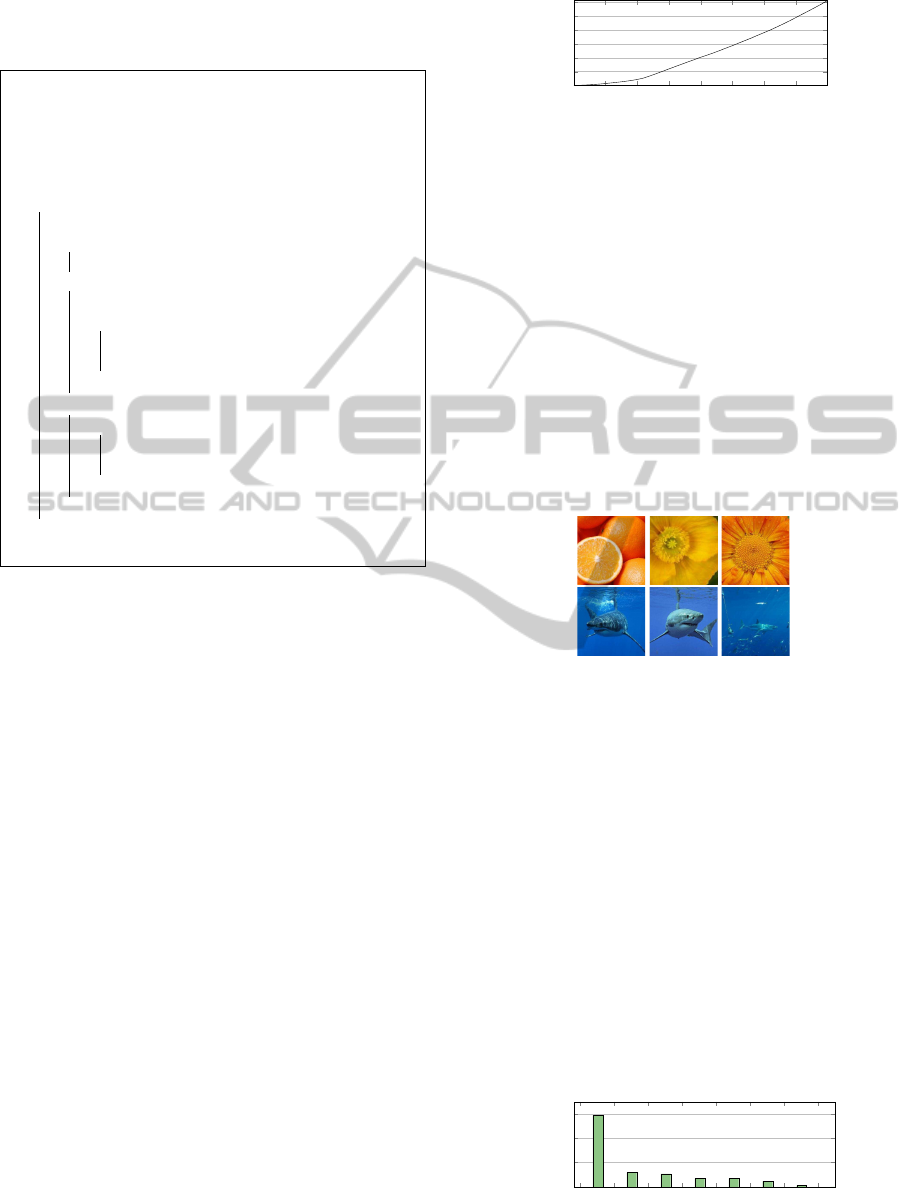
7.1 Index Construction Time
In this experiment we measure the time it requires to
construct indexes of different sizes to determine the
scalability of index construction. We measure the
wall clock time of constructing an index of 40 mil-
lion multidimensional arrays, and measure the time
used between each millionth array We set the thresh-
old th = 500 for this experiment. Figure 3 shows the
result of this experiment.
The first 10 million arrays are indexed much faster
since everything is done in-memory. After this point it
0
5
10
15
20
25
30
35
40
30
60
90
120
150
180
Size of index (in millions)
Time (hours)
Figure 3: Construction time of indexes.
requires accessing the hard drive and thus slows down
significantly. The insertion time is near-linear, only
showing a slight quadratic increase over the course
of several millions insertions. While it is possible to
improve the insertion time, it has not been a primary
focus of this paper.
7.2 Approximate Search Accuracy
Since approximate search is supposed to return an ad-
equate result, it is interesting to measure how good
the result is in general compared to the optimal result.
Figure 4 shows an example of an approximate search
and exact search with an image as the query.
Figure 4: Two search queries on the left, approximate re-
sults in the middle and exact results on the right.
We measure the accuracy of approximate search
with th = 10. We index 100,000 images giving a total
of 22,865 terminal nodes.
We conduct this experiment by searching for 200
queries using the index. For each query we perform
an approximate search for the query. Furthermore, we
sort all 100,000 images in ascending order according
to their exact distance to the query. By finding the po-
sition of the approximate result in the ordered list, we
can determine how close the approximate result was
to the best result. The histogram in Figure 5 shows
that the majority of the results lie within the top 1 %.
This result means that the majority of results from ap-
proximate searches will be similar to results from ex-
act searches.
0 % 1 % 2 % 4 % 8 %
16 %
32 % 100 %
0 %
20 %
40 %
60 %
Distribution of results
Percentage of results in bins
Figure 5: Approximate search accuracy.
ICPRAM2015-InternationalConferenceonPatternRecognitionApplicationsandMethods
196
7.3 Exact Search Performance
Since exact search returns the best possible result, we
are only interested in measuring the performance. To
test the performance of the exact search, we perform
100 search queries on data sets with increasing size
and measure the average amount of nodes which are
read, i.e. how many I/O operations are performed.
This measurement will not depend on hardware or the
implementation and will thus give a more accurate
result than measuring time. We measure the perfor-
mance of exact search with th = 100. The result of
this experiment can be seen in Figure 6.
25 50
100 200 400 800
1,600
3,200
6,400
0 %
20 %
40 %
60 %
80 %
100 %
Size of index (in thousands)
Percentage of nodes read
Figure 6: Amount of nodes read using exact search.
This result shows that the amount (in percent-
age) decreases as the index grows. As we add more
multidimensional arrays, we can obtain a better ap-
proximate result, thus resulting in fewer nodes read
(percentage-wise). In contrast to the result in Fig-
ure 6, a sequential scan will always read all multi-
dimensional arrays (i.e. 100 %). Therefore our index
will decrease the amount of I/O operations. For ex-
tremely large datasets, the percentage of nodes read
should become low. The hyperSAX representation is
better suited for large datasets than for small datasets.
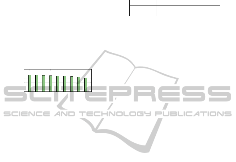
7.4 Time Series Performance
To examine if our representation adds a significant
overhead compared to iSAX, we test it on one-
dimensional arrays, i.e. ordinary time series. By dis-
abling discretization splits, i.e. only doing cardinality
splits, and with a base hyperword type
h
a,a,...,a
i
1
,
where a is the base cardinality and the number of a’s
is the word length, hyperSAX will behave exactly like
iSAX 2.0, with the exception of the utility calculation
for cardinality splits which is a little different.
We perform the test on one million random walk
time series of length 256 with a threshold th = 100.
iSAX 2.0 is simulated with our reduced hyperSAX
implementation and configured with a base cardinal-
ity a = 2 and a word length w = 8. We perform 500
approximate and exact searches, using the same time
series for both indexes. Table 1 shows the results.
The results show that there is only a very slight in-
crease in approximate distance, and a small increase
in the size of the index and the amount of nodes
Table 1: Comparison of the total amount of terminal nodes,
percentage of nodes read using exact search, and the aver-
age approximate distance (AAD).
Nodes total Read AAD
iSAX 15,028 22.5 % 7.03
hyperSAX 18,223 26.9 % 7.32
that are read. Notice how the number of terminal
nodes read is much lower for time series than for im-
ages. We can conclude that the ability to handle mul-
tidimensional arrays in the hyperSAX representation
only adds a small overhead.
8 APPLICATIONS
The hyperSAX representation is created with any
kind of multidimensional data in mind, and using this
representation makes it possible to index and compare
images, GIFs, video, audio or other types of multidi-
mensional data. In this paper we have used images as
examples of indexable multidimensional data, and we
will now introduce an application as a proof of con-
cept.
The application, called “infinite zoom”, makes it
possible to zoom infinitely into images. The goal of
this application is to show that our representation and
index can be used to quickly find similar images based
on an image query.
When we usually zoom into an image using a reg-
ular image viewer, we normally just see fewer and
fewer pixels and the image eventually will become
blurry. Using our infinite zoom, we exchange the
blurry pixels with another image (in higher resolu-
tion), which creates the illusion that we have im-
ages inside images. For this application we use the
CIELAB color space (described in Section 1.1) when
comparing images. We use a collection of images
from the ImageNet database created by Deng et al.
(2009).
We can zoom into any area of the image using the
mouse cursor and scrolling. When we reach a prede-
fined zoom level, we use approximate search to find
an image which has the lowest approximate distance
to the area we are zooming into. We use approximate
search instead of exact search, because speed is essen-
tial (for smoothness) and an approximate result is all
we need. The image found by the approximate search
is then smoothly inserted into the other image, and we
can continue zooming into this new image, thus creat-
ing infinite image zoom. Figure 7 shows an example
of infinite zoom. This example is from searching an
index of size 100,000 where the images are 320×320
and the search area is 32 × 32 pixels.
HyperSAX:FastApproximateSearchofMultidimensionalData
197

Figure 7: Zoom on one image leads to the next image.
9 CONCLUSION
We have developed hyperSAX, a representation and
method for indexing multidimensional arrays. We
have shown that we can use it to index millions of
images, and perform very fast approximate searches
on those images. We have introduced a way to dy-
namically reduce the discretization, i.e. increase word
length, when it is appropriate, rather than providing
a constant word length as required by iSAX and its
derivatives. There is, however, room for improve-
ment, such as improving the splitting policy from Sec-
tion 5.1 to ensure more balanced splits. While com-
paring images using the Frobenius distance measure
may not be optimal, it is still likely to produce good
enough results (from approximate search), as long as
an index contains enough images.
REFERENCES
Andr
´
e-J
¨
onsson, H. (2002). Indexing Strategies for Time Se-
ries Data. Department of Computer and Information
Science, Link
¨
opings universitet.
Bach, J. R., Fuller, C., Gupta, A., Hampapur, A., Horowitz,
B., Humphrey, R., Jain, R., and Shu, C.-F. (1996).
Virage image search engine: an open framework for
image management. In Sethi, I. K. and Jain, R. C.,
editors, Storage and Retrieval for Still Image and
Video Databases IV, volume 2670 of Society of Photo-
Optical Instrumentation Engineers (SPIE) Conference
Series, pages 76–87.
Camerra, A., Palpanas, T., Shieh, J., and Keogh, E. (2010).
iSAX 2.0: Indexing and mining one billion time se-
ries. In Proceedings of the 2010 IEEE International
Conference on Data Mining, pages 58–67. IEEE
Computer Society.
Camerra, A., Shieh, J., Palpanas, T., Rakthanmanon, T., and
Keogh, E. J. (2014). Beyond one billion time series:
indexing and mining very large time series collections
with iSAX2+. Knowl. Inf. Syst., 39(1):123–151.
Cheng, S.-C. and Wu, T.-L. (2006). Speeding up the sim-
ilarity search in high-dimensional image database by
multiscale filtering and dynamic programming. Image
Vision Comput., 24(5):424–435.
Deng, J., Dong, W., Socher, R., Li, L.-J., Li, K., and Fei-
Fei, L. (2009). ImageNet: A Large-Scale Hierarchi-
cal Image Database. In Computer Vision and Pattern
Recognition.
Faloutsos, C., Ranganathan, M., and Manolopoulos, Y.
(1994). Fast subsequence matching in time-series
databases. SIGMOD Rec., 23(2):419–429.
Flickner, M., Sawhney, H., Niblack, W., Ashley, J., Huang,
Q., Dom, B., Gorkani, M., Hafner, J., Lee, D.,
Petkovic, D., Steele, D., and Yanker, P. (1995). Query
by image and video content: the QBIC system. Com-
puter, 28(9):23–32.
Gaede, V. and G
¨
unther, O. (1998). Multidimensional access
methods. ACM Comput. Surv., 30(2):170–231.
Jain, A. K. and Vailaya, A. (1996). Image retrieval using
color and shape. Pattern Recognition, 29(8):1233 –
1244.
Kasson, J. M. and Plouffe, W. (1992). An analysis of
selected computer interchange color spaces. ACM
Trans. Graph., 11(4):373–405.
Keogh, E., Chakrabarti, K., Pazzani, M., and Mehrotra, S.
(2001a). Dimensionality reduction for fast similarity
search in large time series databases. Knowl. Inf. Syst.,
3(3):263–286.
Keogh, E., Chakrabarti, K., Pazzani, M., and Mehrotra, S.
(2001b). Locally adaptive dimensionality reduction
for indexing large time series databases. SIGMOD
Rec., 30(2):151–162.
Lin, J., Keogh, E., Lonardi, S., and Chiu, B. (2003). A sym-
bolic representation of time series, with implications
for streaming algorithms. In Proceedings of the 8th
ACM SIGMOD Workshop on Research Issues in Data
Mining and Knowledge Discovery, pages 2–11. ACM.
Shieh, J. and Keogh, E. (2008). iSAX: Indexing and mining
terabyte sized time series. In Proceedings of the 14th
ACM SIGKDD International Conference on Knowl-
edge Discovery and Data Mining, pages 623–631.
ACM.
Torralba, A., Fergus, R., and Freeman, W. (2008). 80 mil-
lion tiny images: A large data set for nonparamet-
ric object and scene recognition. In IEEE Transac-
tions on Pattern Analysis and Machine Intelligence,
30(11):1958–1970.
Yi, B.-K. and Faloutsos, C. (2000). Fast time sequence
indexing for arbitrary Lp norms. In Proceedings of
the 26th International Conference on Very Large Data
Bases, VLDB ’00, pages 385–394, San Francisco,
CA, USA. Morgan Kaufmann Publishers Inc.
ICPRAM2015-InternationalConferenceonPatternRecognitionApplicationsandMethods
198
