Sparse-input Detection Algorithm with Applications in

Electrocardiography and Ballistocardiography

F. Wadehn

∗,1

, L. Bruderer

∗,1

, D. Waltisberg

, T. Keresztfalvi

and H.-A. Loeliger

Signal and Information Processing Laboratory, ETH Zurich, Gloriastrasse 35, Zurich, Switzerland

Institut fuer Elektronik, ETH Zurich, Gloriastrasse 35, Zurich, Switzerland

Keywords:

Ballistocardiography, Heart Rate Estimation, Hypothesis Test, Factor Graphs, System identiﬁcation, State-

space Models, Maximum likelihood, Maximum a posteriori.

Abstract:

Sparse-input learning, especially of inputs with some form of periodicity, is of major importance in bio-

signal processing, including electrocardiography and ballistocardiography. Ballistocardiography (BCG), the

measurement of forces on the body, exerted by heart contraction and subsequent blood ejection, allows non-

invasive and non-obstructive monitoring of several key biomarkers such as the respiration rate, the heart rate

and the cardiac output. In the following we present an efﬁcient online multi-channel algorithm for estimating

single heart beat positions and their approximate strength using a statistical hypothesis test. The algorithm

was validated with 10 minutes long ballistocardiographic recordings of 12 healthy subjects, comparing it to

synchronized surface ECG measurements. The achieved mean error rate for the heart beat detection excluding

movement artifacts was 4.7%.

1 INTRODUCTION

Cardiovascular diseases are among the leading causes

of death and severe health impairments both in high-

income countries with an aging population, as well

as in developing countries, which are increasingly

adopting western sedentary lifestyles and diet (Yusuf

et al., 2001). Cardiac monitoring appliances range

from high resolution devices such as multi-lead

ECG or the invasive esophageal ECG (Schnittger

et al., 1986) to non-invasive, non-obstructive long

time monitoring systems among which pulse oxime-

try (Yelderman and New Jr, 1983) and ballistocardio-

graphy (BCG) (Alihanka et al., 1981) are the most

prominent. In ballistocardiography, forces exerted by

ventricular blood ejection are measured with force

sensors, usually placed below or inside a mattress on

which patients are lying. These force measurements

can be used to infer heart rates, heart rate variability

and even for getting indications about the cardiac out-

put (Cathcart et al., 1953; Inan et al., 2009). BCG sig-

nals can be interpreted as an overlap of several oscilla-

tions of the body-bed-sensors system. Figure 1 shows

a ﬁltered (see Section 3.1) single channel BCG signal

and heart-beat times (time of R peak in QRS com-

plex), extracted from a synchronized surface ECG.

∗

These two authors contributed equally

Early signal-processing methods for BCG signals

(Watanabe et al., 2005; Mack et al., 2009) concerned

estimation of heart rates averaged over a few sec-

onds using frequency-based methods. These meth-

ods do not provide beat-to-beat resolution or infor-

mation on irregular arrhythmias. Recently, advanced

applications such as heart rate variability analysis or

sleep staging, have brought up the challenging task

of detecting individual heart beats in a BCG signal.

Schemes that rely on a single peak of a, possibly

preprocessed, BCG signal lack robustness for most

applications due to oscillations caused by one heart

beat that decay slowly and overlap with the next heart

beat (Bruser et al., 2011).

A variety of methods, proposed for beat-to-beat

detection are based on, possibly adaptive, template

matching techniques (Shin et al., 2008; Paalasmaa

et al., 2014) or sets of features extracted from the

BCG signal (Friedrich et al., 2010; Bruser et al.,

2011). These approaches have in common that they

are not based on a probabilistic framework and their

performance, which relies on speciﬁc patterns of

troughs and peaks, might decrease, if used with stiff

systems, where oscillations have not sufﬁciently de-

cayed and the following impulse might lead to de-

structive interference. In addition, these algorithms

were developed for single-channel measurement sce-

Wadehn F., Bruderer L., Waltisberg D., Keresztfalvi T. and -A. Loeliger H..

Sparse-input Detection Algorithm with Applications in Electrocardiography and Ballistocardiography.

DOI: 10.5220/0005186600210030

In Proceedings of the International Conference on Bio-inspired Systems and Signal Processing (BIOSIGNALS-2015), pages 21-30

ISBN: 978-989-758-069-7

 2015 SCITEPRESS (Science and Technology Publications, Lda.)

0.5

1.5

Time [s]

BCG a.u.

Figure 1: Filtered single channel BCG signal (solid) with

heart beat positions (red).

narios. Extension of these schemes to process multi-

channel measurements, thus taking advantage of more

information, is not readily possible. In addition the

aforementioned algorithms are tailored to extract in-

stantaneous heart rates from the BCG signals, but do

not recover estimates of the relative strength of heart

beats.

In this paper, we present a robust heart-beat detec-

tion algorithm, which can be used to extract beat-to-

beat estimates (e.g., heart rate or the heart rate vari-

ability) from ballistocardiogram measurements. By

means of an initial training step the method adapts

itself to the present BCG data. Individual heart-

beat then detects beats in a recursive window-based

fashion, using a probabilistic model of the BCG sig-

nal. Core of the model is a state-space model rep-

resentation of the BCG signal and an computation-

ally efﬁcient method for performing hypothesis test-

ing (Reller, 2012). Owing to the explicit modeling of

the BCG heart beat pulses our method is thus robust

when dealing with beat-to-beat interference in the

measurements. Furthermore, the probabilistic treat-

ment allows to quantify the reliability of a poten-

tial heart beat detection and is leveraged for removal

of small artifacts in the signal. Lastly, the estima-

tion algorithm being based on a maximum likelihood

hypothesis-testing procedure, apart from estimates of

heart-beat time also infers the relative magnitude of

beats. Information on the heart beat’s relative magni-

tude might be useful to get indications on the cardiac

output (Kurumaddali et al., 2014).

The paper is structured as follows. At ﬁrst the

BCG signal’s is presented along with our algorithm to

detect individual heart beats and estimate their magni-

tude (Section 2). The employed validation dataset and

necessary pre-processing are then discussed (Section

3), followed by the results (Section 4).

7.6

7.8 8 8.2 8.4

Time [s]

Amplitude a.u.

BCG

4-th order

8-th order

14-th order

Figure 2: One hearbeat period segment of a measured BCG

signal and the estimated state-space model’s outputs, ob-

tained with the presented bootstrap system identiﬁcation

approach. Subspace identiﬁcation with 4-th, 8-th, and 14-

th order model resulted in normalized root-mean-squared-

error (NRMSE) ﬁts

of 32%, 44%, and 52% respectively

evaluted on the training data.

2 ALGORITHM DESCRIPTION

We model BCG signals as a time-shifted sum of beats.

Each beat in turn is modeled as a linear combina-

tion of exponentially-decaying oscillations with addi-

tive white Gaussian noise. Using linear discrete-time

state-space models these signals are described as fol-

lows

= AX

k−1

+ BU

= CX

+ Z

(1)

where the input signal U

represents the heart beat

train, Y

models the measured BCG signal, and Z

∼

N (0,V ) is the observation noise. The heart beat train

is modeled as a scaled non-uniformly spaced Kro-

necker comb

∑

n=0

δ[k − T

] · α

, T

∈ N, (2)

with N heart beats and scaling factors α

, which serve

as indication for the instantaneous cardiac output.

The heart-beat times T

and the scaling factors α

are

unknown and estimated from the BCG signal.

The proposed method used to infer the temporal

pattern of heart-beats, consists of a model-estimation

step, followed by a robust beat-detection algorithm.

The purpose of the model-estimation step is to iden-

tify a suitable state-space model representation in

NRMS is computed as follows

1 −

Y −

Y k

Y − 1/K

∑

k=1

100%,

where Y and

Y represent the stacked BCG measurements

and predictions of the estimated model.

BIOSIGNALS2015-InternationalConferenceonBio-inspiredSystemsandSignalProcessing

Algorithm 1: Sparse-input detection.

1: Pre-processing (Section 3.1)

2: 6σ artifact labeling (Section 2.4)

3: Bootstrapped state-space model identiﬁcation

4: Robust heart-beat detection (Sections 2.2-2.4)

5: Outlier rejection (Section 2.5)

(1) of the current BCG signal. To this end, sub-

space methods were selected, due to their efﬁciency

and their numerical stability (Van Overschee and

De Moor, 1996). Subspace methods (e.g., 4SID) are

based on the idea that an estimate of the state se-

quence ˆx can be directly estimated from input/output

data. Once the state-space sequence is estimated, the

system matrices A,B,C are retrieved using a linear

least squares ﬁt (Ljung, 1998). The covariance V of

the observation noise Z

can be estimated from data

as described in (Van Overschee and De Moor, 1994).

As in our BCG signal model measurements of the

input, the heart-beat times and forces, are not avail-

able, we use a bootstrap method for approximate sys-

tem identiﬁcation: Heart beat excitations are approx-

imated with a signal derived from surface ECG mea-

surements. Speciﬁcally, we assume that the ECG sig-

nal is given for the ﬁrst minute of our trial and use the

times of the R peaks in the QRS complexes as approx-

imate heart-beat times

. In addition, α

≡ 1 is used

for all beats in (2). The synchronized BCG measure-

ments, correspond to the outputs Y

in (1). Currently,

our robust beat-detection algorithm is thus tailored

for setups where a state-space model representation is

known a-priori or setups that allow the use of our sug-

gested bootstrap system identiﬁcation approach. The

input-output system identiﬁcation is performed using

the N4SID algorithm (Van Overschee and De Moor,

1994) with a ﬁxed system order.

Figure 2 demonstrates the approximation of a

single-channel BCG signal using a system order of

4, 8, and 14. The task of heart-beat detection, does

not require the BCG signal to be perfectly represented

by a state-space model: As shown in Section 4, 8-th

models, whose ﬁt to the BCG data Figure 2 is clearly

inferior to higher order models, can still yield nearly

the same error-rate performance for heart-beat detec-

tion. Additionally, lower system orders are more ro-

bust with respect to variations of the BCG model (1)

and demand less computational resources.

2.1 Factor Graph of State-space Model

Since we model the BCG signals probabilistically,

our proposed algorithm relies heavily on probabilis-

tic inference methods. These computations can be

···

Figure 3: Factor graph of initial part of the BCG signal

model.

performed by means of message passing on fac-

tor graphs. Factor graphs describe factorizations of

multi-variable functions(Kschischang et al., 2001).

As shown in (Loeliger et al., 2007), state-space mod-

els can also be represented with factor graphs and ef-

ﬁcient algorithms for probabilistic inference, such as

maximum likelihood estimation and maximum a pos-

teriori estimation can then be derived.

In Forney-style factor-graph (FFG) nota-

tion (Kschischang et al., 2001), boxes represent

factors, whereas edges represent variables. A node

connected to several edges describes a function de-

pending on these variables. As an example, consider

the following factorization of the joint probability

model for Eq. (1), where a length M BCG signal is

observed,

p(y

,...,y

,...,x

,...,u

)

= p(x

) ·

∏

k=1

p(y

k−1

(3)

The initial part of the FFG that corresponds to this fac-

torization is shown in Fig. 3, where the abbreviation

= p(y

i−1

) was employed.

Each block p

in Fig. 3 can be expanded to the

factor shown in Fig. 4. The proposed algorithms are

based on the latter, more detailed, factorization.

Probabilistic inference (e.g., computation of

marginal probability densities for maximum a poste-

riori estimation) is performed by means of message

passing. In message passing algorithms, messages

µ are exchanged between nodes of the graph. Each

node computes output messages based on all incom-

ing messages. Marginal distributions can eventually

be obtained from the product of both messages on an

edge, which face in opposite direction. Central to the

development of our algorithm are forward messages

−→

and backward messages

←−

for state variables

. In particular, these messages represent

−→

) = p(y

,...,y

k−1

,...,u

) (4)

←−

) = p(y

,...,y

k+1

,...,u

). (5)

Sparse-inputDetectionAlgorithmwithApplicationsinElectrocardiographyandBallistocardiography

···

k−1

...

N (0,V )

= y

Figure 4: One sample of the FFG of the linear state-space

model of BCG measurements.

Consequently, the product of these messages corre-

sponds to the probability density

−→

) ·

←−

) = p(y

,...,y

,...,u

). (6)

Given that the current model is a linear function

of Gaussian random variables and unknown deter-

ministic variables, inference of edge variables is per-

formed by means of Gaussian message-passing pre-

sented in (Loeliger et al., 2007). In this case, mes-

sages are Gaussian functionals

−→

(x) = N (x|

−→

) ·

−→

. (7)

These functionals are fully speciﬁed by the mean vec-

tor

−→

m , the covariance matrix

−→

V , and the scale fac-

tor

−→

β =

∞

−∞

−→

µ (x)dx. The computation rules for all

the nodes present in our FFG model (cf. Fig. 4),

are reported in the appendix. For ease of compu-

tations, an equivalent dual parametrization is com-

monly selected for the backward messages

←−

µ : The

messages are described using the inverse covariance

matrix

←−

W , the weighted mean

←−

W ·

←−

m and the scale

factor

←−

γ :=

←−

µ (0).

2.2 Heart-beat Time Estimation

Given a linear state-space model representation in (1)

and a sufﬁciently short multi-channel BCG segment,

the goal is to determine the heart-beat time T . The

main idea consists in performing a hypothesis test

over a time window of N observations and assessing

the likelihood that a heart-beat occurred in exactly one

speciﬁc position. For each point in time k ∈ {1, ..., N}

we have the hypothesis H

stating that all inputs in the

window, except the k-th are zero.

: U

(

, if j = k

0, else

(8)

To determine the position of the input via maximum

likelihood estimation in a hypothesis testing setting,

we will compute the likelihood of each hypothesis,

which is a function of the corresponding input magni-

tude

) = p(y|H

)

= p(y|U

= 0,...,U

= u

,...,U

= 0)

←−

)

(9)

We thus get the likelihood vector

L(~u) with:

L(~u) = (L

),...,L

))

(10)

Since

L is a vector valued function, we will integrate

out each input u

assuming a ﬂat prior over the real or

positive real numbers

to reduce the likelihood func-

tions for each hypothesis to a single value.

∞

←−

)du

= 0.5·

←−

·erfc





−

←−





(11)

To determine the beat position

T , we select the index

of the most likely hypothesis

T = argmax

. (12)

The rationale behind this hypothesis test is to com-

pare how well the signal preceding the assumed input

is described by the state-space model in the absence

of an input and how well the oscillations following

the assumed input, ﬁt to the model’s response to an

input. The robustness of this estimation procedure is

increased if the real heart beat is not too close to the

window’s borders. Estimation of the input magnitude

is done by means of maximum-a-posteriori estimation

using the posterior distribution of u

. The posterior

distribution, is computed taking a ﬂat prior p(u

) as

in (11) and is proportional (i.e., a proportionality fac-

tor independent of u

) to

p(u

,y) =

←−

). (13)

For the ﬁnal algorithm we integrated over the positive

real numbers, which reﬂects the hypothesis that heart beats

are a positive impulses. This assumption leads to likeli-

hoods with less side peaks and thus to a more robust beat

detection

BIOSIGNALS2015-InternationalConferenceonBio-inspiredSystemsandSignalProcessing

Consider the factor graph in Fig. 4 with hidden

states x = (x

,...,x

) and where each variable U

set to 0, thus expressing the probability density

p(y,x|U

= 0,...,U

= 0). (14)

To detect the heart beat time index, messages

←−

) for all possible k are computed in one foward

sweep and one backward sweep. It now follows that

the backward message

←−

) expresses

←−

) = p(y|U

= 0,...,U

= u

,...,U

= 0),

(15)

and using (11), with a ﬂat prior on positive input am-

plitudes, the heart beat estimate

T can be computed

from (12), as well as the input magnitude

MAP

(

←−

≥ 0

←−

< 0

. (16)

Note that computational complexity of this heart beat

time estimation is O(N), thus linear in the length of

the window.

2.3 Window-based Adaptive Beat

Detection

Having established an algorithm to estimate both the

input position and its magnitude given a time win-

dow containing one heart beat, the question that re-

mains is how to choose the windows properly to

cover the whole signal. Our approach was to use an

adaptive jumping window procedure. The bootstrap-

ping begins with a large window e.g. 2s such that

it contains at least one heart beat with high proba-

bility. The estimated position of that heart beat is

denoted as

. Given an estimated heart beat posi-

tion

, place a symmetric window around the posi-

tion where the next beat is assumed to be, denoted

as M

k+1

. Deﬁning an average heart beat period as

HBP

= (

−

k−d

)/d, with d = 3 or d = 5 having

proved to yield good results

, and assuming an initial

HBP of 1 s, we get

k−1

+ HPB

k−1

= [M

− bHBP

k−1

/2c,M

+ bHBP

k−1

/2c].

2.4 Automatic Artifact Detection

Movement artifacts can severely impair BCG mea-

surements and extraction of heart-beat times becomes

impossible. Initial system identiﬁcation and reliable

estimation of heart-beat times both require that cor-

rupted signal segments are detected automatically. To

For the ﬁnal implementation d = 3 was chosen

110 120 130 140

150 160

170

Time [s]

Amplitude a.u.

Figure 5: Prominent artifacts in the BCG signal, are labeled

(shaded) by the 6σ method.

this end, we devise a two-level approach. At ﬁrst,

strong movement artifacts, which are characterized

by a much higher amplitude, are removed after pre-

processing of the measurements. This automatic de-

tection step, labels parts of the signal outside the 6-

sigma band

as artifacts. In a further step, short inter-

vals (< 0.5 s) between two adjacent labeled 6-sigma

bands, were also removed. In this way the BCG

signal is partitioned into useful signal intervals and

movements artifacts, which do not contain informa-

tion about the heart beats as can be seen in Figure 5.

The aforementioned labeling algorithm works

well, when movement artifacts are strong and have

a short duration (e.g. leg movements). In contrast,

a constant presence of small movement artifacts (e.g.

caused by tremor), would result in a very small vari-

ance of the signal and the movement-artifact detec-

tion algorithm would exclude parts of the signal with

slightly elevated amplitude from which the heart beats

could possibly still be extracted. For such signals, we

take advantage of the probabilistic modeling frame-

work: If a corrupted BCG segment is observed and

the model is not able to explain the data well, a sig-

niﬁcant drop in the computed likelihood is observed.

The second level of our automatic artifact detection

method thus drops estimates

T if the average likeli-

hood of the window drops below 50% the prior short-

time average likelihood values. Instead, the estimated

heart-beat time is predicted from past measurements

k−1

+ HPB

k−1

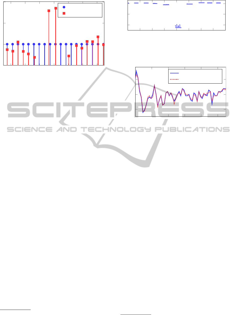
In Figure 6, false estimates are observed from sec-

ond 124 until second 126 caused by a small artifact,

which was not recognized by the 6σ method. How-

ever, the corresponding segment clearly exhibits a sig-

The 6-sigma band is deﬁned as the amplitude values

falling in the interval of ±6σ + µ

Sparse-inputDetectionAlgorithmwithApplicationsinElectrocardiographyandBallistocardiography

120 122 124

126

128 130 132

Time [s]

ECG beats

estimated beats

Figure 6: Heart beat detection and input magnitude estima-

tion. Having no information about the instantaneous cardiac

output from the ECG data, we plot the heart beat magnitude

(black) as a uniform Dirac comb. Movement artifacts at

124s-126s cause midsections, which can be detected from

drops in the likelihood as shown in Figure 7

niﬁcant drop in the average likelihood as shown in

Figure 7.

2.5 Post-processing

Following the recommendations of (Friedrich et al.,

2010), we assume a maximum average heart rate

120 BPM and a minimum heart rate of 30 BPM. Con-

sidering that heart rate measurements are supposed to

occur during rest these bounds are appropriate. These

averaging durations are in accordance with (Bruser

et al., 2011), which states that cardiac monitoring de-

vices can have an update time of up to 10s following

the recommendations of ANSI/AAMI/ISO EC13.

3 MATERIALS AND METHODS

To validate our heart-beat detection method we used

a dataset containing ECG measurements and two-

channel BCG measurements. The dataset comprises

12 healthy subjects (10 male, 2 female) in the age

range of 23-32 years. BCG signals were recorded

for 10 minutes in supine position (facing up), using

piezoelectric pressure sensors placed below the mat-

tress in the area where the torso was assumed to be.

Consequently, torso-ventral displacements, as deﬁned

in (Scarborough et al., 1956), were measured. For val-

idation purposes, a three lead surface ECG synchro-

nized to the BCG signal was recorded. Instantaneous

heart rates ranged from 33 BPM and up to 88 BPM

across all 12 subjects.

The average heart rate is computed by taking the aver-

age over 5 consecutive beats.

Likelihood

Figure 7: Movement artifacts are detected by drops in like-

lihood values. The corrupted signal is recognized and cor-

rected assuming a constant average heart rate. This reﬁne-

ment increases stability and reduces the average heart beat

detection error rate.

290 300 310 320 330 340

Time [s]

Beats per minute

actual heart rate

estimated heart rate

Figure 8: Real ECG-based instantaneous heart rate com-

pared to the instantaneous heart rate extracted from the es-

timated heart-beat times of our method.

3.1 Pre-processing of BCG and ECG

Measurements

Prior to our algorithm, the BCG signal was deci-

mated

from 1000 Hz to 200 Hz primarily to reduce

computational costs and also noise. A 10-th order,

zero-phase bandpass ﬁlter (0.5Hz-30Hz) was com-

bined with a second-order IIR notch ﬁlter at 50 Hz,

using the DSP System toolbox in MATLAB 2014a, to

remove respiratory movements and to remove strong

electrical disturbances at 50 Hz. The ECG signal was

high-pass ﬁltered with a 5-th order Butterworth ﬁlter

at 2 Hz cut-off to remove baseline wandering. Heart

beats were then extracted via peak detection from the

ﬁltered ECG signal.

4 PERFORMANCE EVALUATION

The proposed beat-to-beat estimation algorithm was

validated using ECG measurements as ground truth

in the following way: The ECG heart beat train, con-

taining M heart beats, was split into M segments. The

segments are chosen such that each one contains ex-

actly one heart-beat and their union covers the whole

ECG signal. Given heart beats at times T

k−1

, T

and

Downsampling and anti-alias ﬁltering

BIOSIGNALS2015-InternationalConferenceonBio-inspiredSystemsandSignalProcessing

k+1

, the k-th segment s

is deﬁned as

= [T

− b(T

− T

k−1

)/2c,T

+ b(T

k+1

− T

)/2c].

The estimate

is counted as correct, if exactly one

beat was detected and

∈ [T

− 25ms, T

+ 25ms].

Note that the duration between the electrical activa-

tion and the actual blood ejection displays a varia-

tion of around 8 ms (Friedrich et al., 2010) and thus,

is the maximum precision a beat localization using

BCG measurements can achieve. Assuming an aver-

age window length of 1 s, corresponding to 60 BPM,

the

is required to have a precision of ±2.5%.

Figure 9 shows the heart beat detection error rate

as a function of even system orders

of the state space

model used to describe the BCG signal of subject A.

We can see that too low system orders are not suited

for modeling the BCG signal and lead to very high

error rates. Two channel measurements outperform

single channel measurements for almost all system or-

ders except for very low system orders (2 and 4), for

which it is better to use single channel measurements,

due to the lower complexity of the model required to

describe the single channel measurements. The in-

creasing error rate with system order above 20 could

be hinting to overﬁtting, when system orders are too

high. On the other hand it is also possible that numer-

ical precision issue arise when performing message

passing in factor graphs of state space models of such

high order.

The error-rate performance of the presented

method is evaluated with two 10 minutes long bal-

listocardiogram recordings of 12 healthy subjects, ex-

cluding sections of the signal containing movement

artifacts, which do not provide information about the

heart-beat times. The resulting error rate, averaged

over the test subjects, is 4.7% with a standard er-

ror of the mean of 2.8%. A 14-th order state-space

representation is used to describe the BCG signal.

These performance metrics include one outlier sub-

ject, whose BCG signal contains multiple movement

artifacts, leading to an error rate of 35%. Excluding

the outlier, the mean error rate decreases to 3.4% with

a standard error of the mean of 1.3%.

Automatic artifact detection on the present dataset

results in an average estimation coverage for each

channel, thus the percentage of the signal or windows

not detected as corrupted by movement artifacts. Af-

ter the ﬁrst 6σ labeling method the average coverage

is 95%. Subsequent detection using the likelihood-

based method (see Section 2.4), additionally drops

5% of the windows. Therefore reducing average cov-

erage to around 90%.

Even system orders describe the output signal solely as

a linear combination of exponentially decaying oscillations

2 4

8 10 12 14

18 20 22 24

System order

Error rate [%]

one channel

two channels

Figure 9: Heart beat detection error rate for subject A as

a function of the system order for single and two-channel

measurements.

Figure 8 compares the beat-to-beat (instanta-

neous) heart rate extracted from ECG and from the

estimates

T of the suggested method. The estimated

heart-beat times reveal even small ﬂuctuations in the

beat-to-beat times. The average interval error be-

tween actual heart beats (ECG) and estimated heart

beats was computed according to (Friedrich et al.,

2010) resulting in an average heart beat interval error

of 33.1 ms. Note that the average heart beat detection

error rate, introduced above, is better suited to assess

our algorithm, as it identiﬁes single heart beats (i.e.,

beat detection and time

) and not the intervals be-

tween heart beats.

The heart beat detection algorithm takes around

60 s to estimate instantaneous heart rates in a 10 min-

utes long two-channel BCG signal using MATLAB

R2014a on a 3.33 GHz, 8 GB personal computer, in-

cluding system estimation, loading of data and pre-

processing. The pure heart beat estimation takes

around 35 s, for the 10 minutes long BCG sequences,

thus when allowing a small delay (e.g. 5 s) and a start

up-time for 30 s the algorithm could run in real time,

especially when implemented in faster programming

languages such as C/C++.

5 DISCUSSION AND

CONCLUSIONS

We have presented a novel method to extract beat-

to-beat data from ballistocardiograms. Given an es-

timated or known linear state-space model represen-

tation of the ballistocardiogram signal, heart beats are

extracted from measured data using a robust input-

estimation algorithm. We have shown that additional

measurement channels (i.e., multiple sensors) yield

signiﬁcant performance improvements in terms of

error-rate and robustness. Owing to the model-based

approach, the method can correctly extract movement

Sparse-inputDetectionAlgorithmwithApplicationsinElectrocardiographyandBallistocardiography

artifacts from measured data and recognize when beat

detection is impaired or not possible. Validation of the

method on ballistocardiogram measurements of 12

healthy subjects showed 4.7% average beat-detection

error rate. The presented algorithm lends itself to ap-

plication on a multitude of almost periodic signals,

especially in cardiology.

Currently, the algorithm at ﬁrst adapts itself to a

speciﬁc BCG signal, as described in Section 2. It

is likely that alterations of the system (e.g., changed

body position) will trigger the likelihood-based arti-

fact detection routine (see Section 2) and a new sys-

tem identiﬁcation step will become necessary. How-

ever, in the present dataset, subjects were laying still

and this issue was not observed.

A further complication, which was also not ob-

served in the current dataset, may arise when strong

heart-rate variability occurs. The window-based ap-

proach may either select a window where no beat

is present or a window with two beats. In the ﬁrst

case, a false-positive beat will be detected, while in

the other case, the algorithm will miss a beat and

make a false-negative error. This issue could be ad-

dressed by considering the relative likelihood value

of a beat estimate to the other indices with large like-

lihood values and deciding if two beats are present or

none. Also schemes which run the window-based de-

tection schemes multiple times and each time includ-

ing the currently detected beats and models on heart-

rate variability might mitigate these type of errors.

Blind system identiﬁcation i.e., estimation of the

state-space model solely on BCG measurements,

would facilitate applicability of the current method.

As a consequence, the resulting method would not

require ECG measurement equipment and would be

able to adapt to varying external factors (e.g., sleeping

position). Moreover, investigating on the relation be-

tween the estimated input magnitude and the instan-

taneous cardiac output, which is a key biomarker for

various cardiovascular diseases, seems to be a promis-

ing direction for future research.

A further enhancement can be achieved by multi-

plying the hypothesis likelihood with a Gaussian win-

dow, centered around the assumed input, serving as

a prior on the heart beat position. This reﬁnement

signiﬁcantly improves error rates, when the BCG sig-

nal is hardly contaminated by movement artifacts. On

the other hand when the signal contains several move-

ment artifacts, it is better not to assume any prior on

the beat position to avoid error propagation. To deal

with a general BCG signal, possibly heavily contam-

inated with artifacts, the Gaussian window was omit-

ted in the performance evaluation in subsection 4.

Table 1: Performance metrics.

Metric Unit Value

Signal duration min 10

Coverage 6-σ labeling % 95

Coverage likelihood drop labeling % 90

HB detection error rate % 4.7

HB interval error ms 33.1

ACKNOWLEDGEMENTS

The authors would like to thank Nour Zalmai for valu-

able feedback concerning the sparse-input learning al-

gorithm. Furthermore we highly appreciated the valu-

able discussions with Dr. med. Reto Wildhaber re-

garding the cardiovascular system.

REFERENCES

Alihanka, J., Vaahtoranta, K., and Saarikivi, I. (1981). A

new method for long-term monitoring of the ballisto-

cardiogram, heart rate, and respiration. Am J Physiol,

240(5):R384–92.

Bruser, C., Stadlthanner, K., de Waele, S., and Leonhardt,

S. (2011). Adaptive beat-to-beat heart rate estimation

in ballistocardiograms. IEEE Transactions on Infor-

mation Technology in Biomedicine,, 15(5):778–786.

Cathcart, R. T., Field, W. W., and Richards Jr, D. W. (1953).

Comparison of cardiac output determined by the bal-

listocardiograph (nickerson apparatus) and by the di-

rect ﬁck method. Journal of Clinical Investigation,

32(1):5.

Friedrich, D., Aubert, X., Fuhr, H., and Brauers, A.

(2010). Heart rate estimation on a beat-to-beat ba-

sis via ballistocardiography-a hybrid approach. In En-

gineering in Medicine and Biology Society (EMBC),

2010 Annual International Conference of the IEEE,

pages 4048–4051. IEEE.

Inan, O., Etemadi, M., Paloma, A., Giovangrandi, L., and

Kovacs, G. (2009). Non-invasive cardiac output trend-

ing during exercise recovery on a bathroom-scale-

based ballistocardiograph. Physiological measure-

ment, 30(3):261.

Kschischang, F. R., Frey, B. J., and Loeliger, H.-A. (2001).

Factor graphs and the sum-product algorithm. In-

formation Theory, IEEE Transactions on, 47(2):498–

519.

Kurumaddali, B., Marimuthu, G., Venkatesh, S. M., Suresh,

R., Syam, B., and Suresh, V. (2014). Cardiac output

measurement using ballistocardiogram. In The 15th

International Conference on Biomedical Engineering,

pages 861–864. Springer.

Ljung, L. (1998). System identiﬁcation. Springer.

Loeliger, H.-A., Dauwels, J., Hu, J., Korl, S., Ping, L., and

Kschischang, F. R. (2007). The factor graph approach

BIOSIGNALS2015-InternationalConferenceonBio-inspiredSystemsandSignalProcessing

to model-based signal processing. Proceedings of the

IEEE, 95(6):1295–1322.

Mack, D. C., Patrie, J. T., Suratt, P. M., Felder, R. A., and

Alwan, M. (2009). Development and preliminary val-

idation of heart rate and breathing rate detection using

a passive, ballistocardiography-based sleep monitor-

ing system. Information Technology in Biomedicine,

IEEE Transactions on, 13(1):111–120.

Paalasmaa, J., Toivonen, H., and Partinen, M. (2014). Adap-

tive heartbeat modelling for beat-to-beat heart rate

measurement in ballistocardiograms. IEEE Journal

of Biomedical and Health Informatics,, PP(99):1–1.

Reller, C. (2012). State-space methods in statistical signal

processing: New ideas and applications. PhD thesis,

ETH Zurich.

Scarborough, W. R., Talbot, S. A., Braunstein, J. R., Rap-

paport, M. B., Dock, W., Hamilton, W., Smith, J. E.,

Nickerson, J. L., and Starr, I. (1956). Proposals for

ballistocardiographic nomenclature and conventions:

revised and extended report of committee on ballis-

tocardiographic terminology. Circulation, 14(3):435–

450.

Schnittger, I., Rodriguez, I. M., and Winkle, R. A. (1986).

Esophageal electrocardiography: a new technology

revives an old technique. The American journal of

cardiology, 57(8):604–607.

Shin, J., Choi, B., Lim, Y., Jeong, D., and Park, K. (2008).

Automatic ballistocardiogram (bcg) beat detection us-

ing a template matching approach. In Engineering

in Medicine and Biology Society, 2008. EMBS 2008.

30th Annual International Conference of the IEEE,

pages 1144–1146.

Van Overschee, P. and De Moor, B. (1994). N4sid:

Subspace algorithms for the identiﬁcation of com-

bined deterministic-stochastic systems. Automatica,

30(1):75–93.

Van Overschee, P. and De Moor, B. (1996). Subspace iden-

tiﬁcation for linear systems: Theory, implementation.

Methods.

Watanabe, K., Watanabe, T., Watanabe, H., Ando, H.,

Ishikawa, T., and Kobayashi, K. (2005). Noninva-

sive measurement of heartbeat, respiration, snoring

and body movements of a subject in bed via a pneu-

matic method. Biomedical Engineering, IEEE Trans-

actions on, 52(12):2100–2107.

Yelderman, M. and New Jr, W. (1983). Evaluation of pulse

oximetry. Anesthesiology, 59(4):349–351.

Yusuf, S., Reddy, S.,

Ounpuu, S., and Anand, S. (2001).

Global burden of cardiovascular diseases part i: gen-

eral considerations, the epidemiologic transition, risk

factors, and impact of urbanization. Circulation,

104(22):2746–2753.

APPENDIX

Message Passing

Measurements are plugged into the factor graph, re-

sulting in Dirac delta messages. Let X

∈ R

and

∈ R

←−

)=δ(y

− y

obs

)

Sum-product message passing through the sum-factor

(

+ Z

←−

−1

←−

−1

←−

−→

= 1

←−

( ˜y

)=(2π)

−

det(V )

−

( ˜y

−y

)

−1

( ˜y

−y

)

←−

(0) =

←−

= (2π)

−

det(V )

−

−1

←−

Forward Message Passing

Forward message passing corresponds to Kalman ﬁl-

tering in the state space model. The update equations

are

−→

←−

−C

−→

)

−→

−

−→

−1

←−

−→

V : =

←−

−→

m : =C

−→

←−

−→

←−

(2π)

· det(V )

−

−1

−→

Sparse-inputDetectionAlgorithmwithApplicationsinElectrocardiographyandBallistocardiography

−→

k+1

−→

k+1

−→

k+1

−→

Backward Message Passing

Backward message passing corresponds to Kalman

smoothing in the state space model. The update equa-

tions are

←−

(2π)

det(

←−

)

←−

Rejoining Messages

To determine the marginal distribution of U

we com-

bine the forward and backward messages.

←−

k+1

←−

k+1

−

−→

←−

k+1

←−

k+1

−→

←−

k+1

−→

←−

k+1

For the heart beat estimation problem we assume that

the input is scalar.

←−

(2π)

n−1

det(

←−

)

det(

←−

)

−

←−

V : =

←−

− B

←−

BIOSIGNALS2015-InternationalConferenceonBio-inspiredSystemsandSignalProcessing