New Spectral Representation and Dissimilarity Measures Assessment for
FTIR-spectra using Unsupervised Classification
Francisco Pe˜naranda
1
, Fernando L´opez-Mir
1
, Valery Naranjo
1
, Jes´us Angulo
2
, Lena Kastl
3
and Juergen Schnekenburger
3
1
Instituto Interuniversitario de Investigaci´on en Bioingenier´ıa y Tecnolog´ıa Orientada al Ser Humano,
Universitat Polit`ecnica de Valencia, Valencia, Spain
2
CMM-Centre de Morphologie Math´ematique, Math´ematiques et Syst`emes, MINES Paristech, Fontainebleau, France
3
Biomedical Technology Center, University of Muenster, D-48149, Muenster, Germany
Keywords:
FTIR-spectroscopy, Hyperspectral Imaging, Dissimilarity Measures, Clustering, Cancer.
Abstract:
In this work, different combinations of dissimilarity coefficients and clustering algorithms are compared in or-
der to separate FTIR data in different classes. For this purpose, a dataset of eighty five spectra of four types of
sample cells acquired with two different protocols are used (fixed and unfixed). Five dissimilarity coefficients
were assessed by using three types of unsupervised classifiers (K-means, K-medoids and Agglomerative Hier-
archical Clustering). We introduce in particular a new spectral representation by detecting the signals’ peaks
and their corresponding dynamics and widths. The motivation of this representation is to introduce invariant
properties with respect to small spectra shifts or intensity variations. As main results, the dissimilarity mea-
sure called Spectral Information Divergence obtained the best classification performance for both treatment
protocols when is used over the proposed spectral representation.
1 INTRODUCTION
Early diagnosis of cancer is one of the most effective
ways for reducing the mortality of this disease (Carter
et al., 2013). However, the classification of healthy
and unhealthy tissue in some stages of the pathol-
ogy is a difficult task using current optical imaging
or visual inspection. Chemical images have been
developed to define not only anatomical structure,
but also molecular properties (Petibois and Deleris,
2006). This is the case of Fourier Transform Infra-
Red (FTIR) images, which are based on the amount of
light that molecules absorb in the range of IR wave-
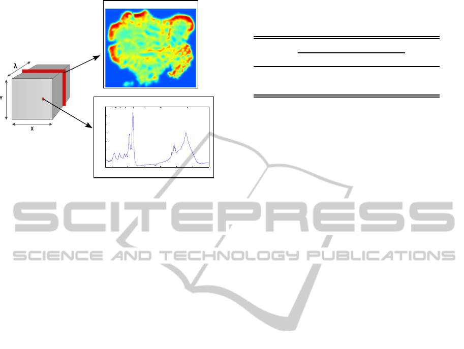
lengths or wavenumbers. FTIR images are cubes of
hyperspectral signals where one 2D image represents
the absorption of the tissue for a specific wavenum-
ber and if a spatial point (x
0
,y
0
) is fixed, a particular
spectrum is obtained (Fig. 1).
FTIR spectroscopy, applied to the diagnosis of
cancer, is still a developing research area, dating the
pioneer studies from the beginning of this century
(Kendall et al., 2009). In this context, the majority
of studies only considers the Euclidean distance as a
measure of dissimilarity for any kind of classification
task. For example, in (Krafft et al., 2008) and (Nal-
lala et al., 2014), unsupervised classification is used
for segmentation purposes with this type of measure
and K-means algorithm. Another point that has not
been questioned in the related literature is the election
of the clustering algorithm. The only publication that
tries to compares different performances of clustering
algorithms (K-means, Fuzzy C-means and Agglomer-
ative Hierarchical Clustering) is (Lasch et al., 2004).
Unfortunately, all these studies only analyse the clas-
sification performance in a qualitative way.
In this work the ability to arrange different cells
spectra by combining five dissimilarity coefficients
with three unsupervised classifiers is evaluated by
means of objective indices. The raw data and a new
spectral representation based on main features of the
signal are analysed as inputs of these algorithms.
Section 2 defines the materials, the dissimilar-
ity coefficients and clustering techniques used in this
work as well as the proposed new spectral representa-
tion. In Section 3, the results of the classification task
are shown and they are discussed in Section 4. Fi-
nally, Section 5 presents the conclusions of this work.
172
Peñaranda F., López-Mir F., Naranjo V., Angulo J., Kastl L. and Schnekenburger J..
New Spectral Representation and Dissimilarity Measures Assessment for FTIR-spectra using Unsupervised Classification.
DOI: 10.5220/0005188001720177
In Proceedings of the International Conference on Bio-inspired Systems and Signal Processing (BIOSIGNALS-2015), pages 172-177
ISBN: 978-989-758-069-7
Copyright
c
 2015 SCITEPRESS (Science and Technology Publications, Lda.)

10 9 8 7 6 5 4 3
wavelength (µm)
1000 1500 2000 2500 3000 3500 4000
0
0.1
0.2
0.3
0.4
0.5
0.6
wavenumber (cm
1
)
absorbance
1663 cm
-1
Figure 1: FTIR images. Left: Data cube associated to
the hyperspectral image. Right, top: Pseudocolor image
representing the spatial absorbance values for a constant
wavenumber. Right, bottom: Absorbance spectrum corre-
sponding to a specific spatial point of the data cube.
2 METHOD
2.1 Spectral Data
Eighty-five spectra of different types of cells were
measured using CaF
2
as substrates for the culture and
preparation. The cells are divided in four groups: A-
375 and SK-MEL-28 cell samples are two skin cancer
cell types and HaCaT and NIH-3T3 cell samples rep-
resent the two major cellular skins: keratinocytes and
fibroblasts. Fifty-eight cell samples were fixed with
glutaraldehyde, dehydrated with ethanol and air dried
before measurements. Twenty-seven were unfixed in
cell media and air dried immediately before measur-
ing. Table 1 summarises this information.
The spectra were measured in transmission mode
with an IFS 66v/S spectrometer from Bruker Optics
equipped with a SiC global source and a DLaTGS
detector. The acquisition software subtracted auto-
matically the reference spectrum of the associated
CaF
2
window. Each spectrum was acquired between
wavenumbers 1000-4000 cm
−1
with a resolution of 1
cm
−1
, what results in a vector of 3000 components.
In the pre-processing steps absorbance (A) was
calculated from transmittance (T) as A = −log
10
(T)
and a Savitzky-Golay smoothing filter with a win-
dow of 31 points and third-order fitted polynomial
was applied (Rinnan et al., 2009). Finally, each spec-
tral vector was normalised with its Euclidean norm as
x
norm
= x/||x|| (Baker et al., 2008). The normalisa-
tion is necessary to minimise possible artefacts during
the acquisition process of the IR light (Lasch, 2012).
Table 1: Number of available spectral samples for each kind
of cancerous (A-375, SK-MEL-28) and normal (Ha-CaT,
NIH-3T3) cells, divided by type of treatment protocol.
Type
Cancer Normal
Total
A SK HA NIH
Fixed 11 22 10 15 58
Unfixed 11 8 8 0 27
2.2 Dissimilarity Measures
Five dissimilarity coefficients were implemented us-
ing Matlab software. A distance matrix (d
i, j
) was ob-
tained, where each value measures the dissimilarity
between signals i and j according to the selected co-
efficient. This distance matrix is symmetric with val-
ues equal to zero in the diagonal and positive values
out of it. The dissimilarity coefficients assessed were:
• Euclidean Distance. It is the most intuitive and
fastest measure which is computed by the root of
the square differences between the coordinates of
a pair of vectors.
• City Block Distance. Also known as Manhattan
distance, it measures the absolute difference be-
tween the coordinates of two spectral vectors.
• Cosine Distance. It is computed as 1 minus the
cosine between two spectral vectors. Hence, two
spectral vectors with a zero angle between them
has a cosine distance equals to zero.
• Correlation Distance. It is a special case of an-
gular separation standardised by centring the co-
ordinates on its mean and is computed as 1 minus
the correlation coefficient.
• Spectral Information Divergence (SID). It is
based on Spectral Information Measure (SIM)
(Chang, 2003) that considers the inter-band vari-
ability as a result of uncertainty incurred by ran-
domness and models the spectral vector as a prob-
ability distribution. In the context of informa-
tion theory, SID is the symmetrised version of
Kullback-Leibler divergence, which measures the
relative entropy provided by each spectral vector.
2.3 Gaussian Model
A new representation of the spectrum is introduced
to take into account the most relevant information of
its the main peaks. The regional maxima of the sig-
nal were found automatically and only the absolute
maxima in a neighbourhood of twenty samples were
selected to discard noisy maxima. In the peaks ob-
NewSpectralRepresentationandDissimilarityMeasuresAssessmentforFTIR-spectrausingUnsupervisedClassification
173

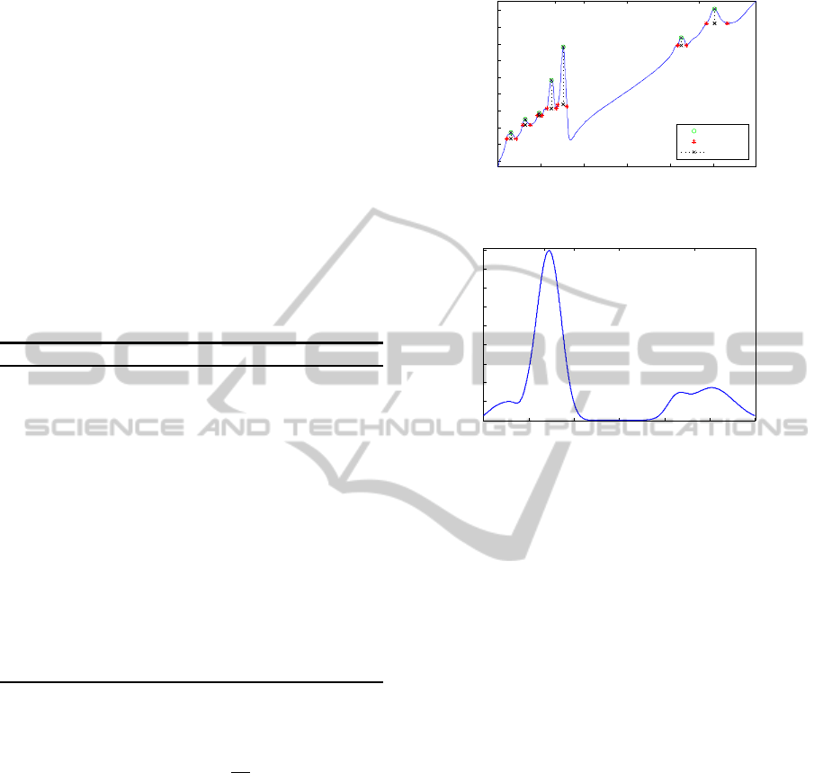
tained after this filter, the dynamic of each peak and
its width were computed.
Algorithm 1 summarises the process for obtain-
ing these two features. A reconstruction by dilation
was carried out in the spectrum where h was a con-
stant value for each iteration (Soille, 2002). The val-
ues of h spanned from 0 to h
max
, which is equal to
the difference between the maximum and the min-
imum of each spectrum, and ∆h = h
max
/100. The
residue was computed and the cross-by-zero around
each peak calculated for obtaining two wavenumbers.
If these wavenumbers fulfilled some restrictions with
the wavenumbers of the maximum neighbours, the h
value was considered as the dynamic and the width
was extracted directly as the difference of the two
wavenumbers. Fig. 2a shows, in a specific signal, the
properties of each peak obtained with this process.
Algorithm 1: Extraction of peaks’ dynamic and width.
x = spectrum with relevant maxima detected at
wavenumbers A
1
,...,A
n
For each peak (i = 1 : n)
For h = 0 : (h
max
/100) : h
max
Y = reconstruction (x, x-h)
R = x - Y
Follow the two cross-by-zero in R around the
peak to obtain two wavenumbers (w
1
,w
2
)
If (w
1
> A
i−1
AND w
2
< A
i+1
)
Dynamic
i
= h
Width
i
= w
2
− w
1
Go to next peak
End if
End h
End peak
A Dirac delta function with an intensity equals
to the corresponding dynamic was positioned in each
peak’s wavenumber. Each Dirac delta was convolved
with a Gaussian function: e
−
w
2
2σ
2
, where w is the
wavenumber variable and σ = width
peak
. Finally, the
resulting convolutions were added to form an equiv-
alent spectral representation that contains relevant in-
formation of the original spectrum, Fig. 2b.
The aim of this model is to represent the most im-
portant information within the signal in a more ro-
bust and simpler way. Finding only the features of
the principal peaks the noise due to different sources
as scattering, which causes additive and multiplica-
tive intensity artefacts, is reduced. By convolving the
Dirac deltas with an adaptive Gaussian function, the
model tries to be more robust against small changes or
shifts in the position of the peaks, which can also be
produced by scattering effects and even imperfections
in the spectroscopic light sensor.
6 5 4 3
wavelength (µm)
1500 2000 2500 3000 3500 4000
0.008
0.01
0.012
0.014
0.016
0.018
0.02
0.022
0.024
0.026
wavenumber (cm
−1
)
absorbance
Amplitude
Width
Dynamic
(a) Peaks properties of the original spectra.
6 5 4 3
wavelength (µm)
1500 2000 2500 3000 3500 4000
0
1
2
3
4
5
6
7
8
9
x 10
−3
wavenumber (cm
−1
)
absorbance
(b) Gaussian model representation.
Figure 2: Proposed spectral Gaussian model.
2.4 Unsupervised Classification
There is a wide variety of clustering algorithms with
different characteristics due to their distinct ways
to group a dataset and the measure of similarity or
dissimilarity is data dependent (Bandyopadhyay and
Saha, 2013). Hence, it is important to compare the
performance of different combinations of classifica-
tion methods and distance coefficients.
Three types of clustering algorithms were used to
assess how suitable the studied dissimilarity measures
are for correctly discriminating the spectral samples.
In these techniques, the number of clusters k must be
specified (k = 4 in fixed and k = 3 in unfixed cells).
• K-means (KM). It is the most popular cluster-
ing algorithm used in many fields of interest. It
is a partitioning algorithm that divides data into
k subsets represented by their centroids, which
are calculated by the mean or weighted average
of the cluster members. The iterative partitioning
minimises an objective function based on the Eu-
clidean norm that represents the total intra-cluster
variance. There are a lot of variations of this algo-
rithm in the literature (Berkhin, 2006; Jain, 2010).
In this algorithm only the former four distances
described in Sec. 2.2 can be implemented due to
the definition of the objective function.
BIOSIGNALS2015-InternationalConferenceonBio-inspiredSystemsandSignalProcessing
174

• K-medoids (Kmd). It is another popular partition-
ing clustering algorithm. This is an extension of
KM where the concept of medoid (a representa-
tive data point from the dataset) is used instead
of the centroid. Kmd minimizes a sum of pair-
wise dissimilarities instead of a sum of squared
Euclidean distances (Bandyopadhyay and Saha,
2013), so, the five studied distances can be imple-
mented. Kmd is more robust to noise and outliers
than KM because the computation of medoids is
dictated by the location of a predominant fraction
of points inside a cluster (Berkhin, 2006).
• Agglomerative Hierarchical Clustering (AHC).
It builds a hierarchy of clusters starting with one-
point (singleton) clusters and recursively merges
two or more of the most similar clusters as one
moves up the hierarchy. The linkage clustering
technique is a non-iterative process based on a lo-
cal connectivity criterion. The four methods of
linkage used in this paper differ in the definition
of the distance between clusters:
– Single linkage utilizes the smallest distance be-
tween points in the two clusters.
– Complete linkage makes use of the largest dis-
tance between points in the two clusters.
– Average linkage uses the average distance be-
tween all pairs of points in any two clusters.
– Weighted average linkage uses a recursive def-
inition for the distance between two clusters.
2.4.1 Performance Measures
Three indices were used to assess the performance of
the clustering algorithms with the dissimilarity coef-
ficients. The first index, the Overall Accuracy (OA),
measures the accuracy to group the spectra in their
correct type of cell and is defined as:
OA(%) =
∑
k
i=1
c
ii
∑
k
i=1
∑
k
j=1
c
ij
· 100, (1)
where c
ij
is the number of spectra classified as class
j and referenced as class i. The second group of in-
dices evaluates the results from a diagnostic point of
view. These are the well known Sensitivity (Sn) and
Specificity (Sp), defined as:
Sn(%) =
TP
TP+ FN
· 100, Sp(%) =
TN
TN + FP
· 100
(2)
where TP are the True Positives (cancer cells cor-
rectly classified), FN are the False Negatives (cancer
cells incorrectly classified), TN are the True Nega-
tives (normal cells correctly classified) and FP are the
False Positives (normal cells incorrectly classified).
3 RESULTS
The different combinations of dissimilarity measures
and clustering algorithms using the pre-processed raw
spectra and the proposed Gaussian model are evalu-
ated in Table 2. Cell samples were studied separately
depending on their chemical treatment protocol be-
cause it has a crucial influence in the properties of
spectra. Results for fixed cells are presented in the top
part of Table 2 and unfixed cells in the bottom part.
Although the four described linkage methods for
AHC were implemented, only the results for single
linkage are shown because they obtained the highest
OA. Sn and Sp are shown because they give impor-
tant information for diagnosis; nevertheless, OA is the
chosen index to select the best combinations because
it condenses the efficiency of the classifications in the
actual type of cells, not only considering if they are
normal or pathological (Table 1). For each treatment
protocol, the highest OA is highlighted.
In fixed cells, if the pre-processed raw spectra is
used, the best similarity measure is the city block
distance with KM as well as Kmd, although the Eu-
clidean distance also has a close efficiency with Kmd
and AHC. On the other hand, the Gaussian model has
an equivalent OA if Kmd is used with SID, although
the cosine distance with KM and Kmd has a slightly
low performance. The Sn values for the highest OA
are equivalent in the two spectral representations but
the Gaussian model has a higher Sp.
In unfixed cells, the results of the Gaussian model
looks impressive since the 100% of OA is obtained for
any dissimilarity measure using Kmd and using cosine
and correlation distance with KM. In the case of the
pre-processed raw spectra, the results are also very
satisfactory for Kmd with Euclidean and city block
distance. The Sn and Sp are also maximum for the
best OA obtained with the Gaussian model. However,
the performance results can be very low for some
combinations, mainly the Sp index.
4 DISCUSSION
The performance values seems to be really promising
for some combinations, but the results must be taken
with caution mainly due to the small number of avail-
able samples, especially in unfixed cells.
Another related problem is the differentnumber of
cell types for each kind of treatment protocol (Table
1). In fixed cells, the number of SK-MEL-28 (22 sam-
ples) is higher than the rest of cell types, what might
have affected the value of OA because the classifica-
tion of this type of cells has a higher weight in its cal-
NewSpectralRepresentationandDissimilarityMeasuresAssessmentforFTIR-spectrausingUnsupervisedClassification
175

Table 2: Results of performance of the different combinations of dissimilarity measures and clustering algorithms for the two
types of treatment protocols (Above: Fixed, Below: Unfixed), using the pre-processed raw spectra and the proposed Gaussian
model. (OA: Overall Accuracy, Sn: Sensitivity, Sp: Specificity).
Fixed
Euclidean City Block Cosine Correlation SID
K-means
Raw Spectra
OA 79.3 93.1 79.3 81
Sn 100 93.9 100 100 -
Sp 100 100 100 100
Gaussian
OA 79.3 89.7 91.4 82.8
Sn 100 100 93.9 93.9 -
Sp 100 100 92 72
K-medoids
Raw Spectra
OA 91.4 93.1 81 81 79.3
Sn 93.9 93.9 100 100 100
Sp 100 100 100 100 100
Gaussian
OA 81 89.7 91.4 82.8 93.1
Sn 100 100 93.9 93.9 93.9
Sp 100 100 92 72 96
Hierarchical
Raw Spectra
OA 91.4 82.8 81 69 72.4
Sn 84.8 100 100 90.9 100
Sp 100 100 100 40 80
Gaussian
OA 74.1 72.4 65.5 50 65.5
Sn 84.8 84.8 84.8 84.8 84.8
Sp 100 100 44 4 48
Unfixed
Euclidean City Block Cosine Correlation SID
K-means
Raw Spectra
OA 59.3 96.3 59.3 59.3
Sn 84.2 94.7 57.9 84.2 -
Sp 0 100 100 0
Gaussian
OA 59.3 59.3 100 100
Sn 84.2 57.9 100 100 -
Sp 0 100 100 100
K-medoids
Raw Spectra
OA 96.3 96.3 59.3 59.3 59.3
Sn 94.7 94.7 84.2 84.2 84.2
Sp 100 100 0 0 0
Gaussian
OA 100 100 100 100 100
Sn 100 100 100 100 100
Sp 100 100 100 100 100
Hierarchical
Raw Spectra
OA 59.3 59.3 59.3 59.3 59.3
Sn 57.9 57.9 57.9 84.2 57.9
Sp 100 100 100 0 100
Gaussian
OA 59.3 55.6 74.1 66.7 77.8
Sn 57.9 78.9 100 57.9 68.4
Sp 100 0 12.5 100 100
culation. In unfixed cells, the number of samples of
different cell types is quite balanced, but the number
of cancer (19 samples) and normal cells (8 samples)
is very different, so in this case the unbiased indices
are Sn and Sp. This fact is more important for Sp in-
dex because if the separation of the 8 normal samples
BIOSIGNALS2015-InternationalConferenceonBio-inspiredSystemsandSignalProcessing
176

fails its value is really low or even zero.
In spite of these problems, the obtained results are
valuable because they demonstrate that the election
of the dissimilarity measure along with the clustering
algorithm is important for the classification perfor-
mance. This fact should be taken into account in an-
other clustering applications of FTIR data, where only
the Euclidean distance is commonly utilised (Sec. 1).
5 CONCLUSIONS
A methodology for studying the ability of five dissim-
ilarity coefficients to correctly separate hyperspectral
data was carried out. For this purpose three different
clustering algorithms were used to gather eighty five
spectra in their corresponding types of cell. These
spectra belonged to two different groups due to the
two different protocols used in the acquisition step.
As a novelty, a new spectral representation model
has been described. This method extracts the main
features enclosed in the principal peaks of the spec-
trum and translates them into a signal that can be more
robust against scattering and sensor’s artefacts.
As main conclusion of this study, not only the op-
timal dissimilarity measure is data dependent, but also
the optimal clustering algorithm. It is necessary to ex-
tend this study to new spectral data to be able to gener-
alise the results. Nevertheless, the Spectral Informa-
tion Divergence has obtained the best overall results
in the classification task when is applied over the pro-
posed Gaussian model in both treatment protocols.
The future steps will be the comparison of other
dissimilarity coefficients and more complex cluster-
ing algorithms in new FTIR datasets containing more
samples. As inputs of the algorithms, new ways to
represent the main information of spectra (PCA and
Sparse Representation) will be studied and compared
with the proposed Gaussian model, which will be im-
proved to contain other significant signal properties.
ACKNOWLEDGEMENTS
This research has been supported by the European
Commission through the Framework Seven project
MINERVA (317803; www.minerva-project.eu).
REFERENCES
Baker, M., Gazi, E., Brown, M., Shanks, J., Gardner, P., and
Clarke, N. (2008). FTIR-based spectroscopic analysis
in the identification of clinically aggressive prostate
cancer. Br J Cancer, 99(11):1859–66.
Bandyopadhyay, S. and Saha, S. (2013). Unsuper-
vised Classification: Similarity Measures, Classi-
cal and Metaheuristic Approaches, and Applications.
Springer.
Berkhin, P. (2006). A survey of clustering data mining tech-
niques. In Grouping multidimensional data, pages 25–
71. Springer.
Carter, H. B., Albertsen, P., Barry, M., Etzioni, R., Freed-
land, S., Greene, K., Holmberg, L., Kantoff, P.,
Konety, B., Murad, M., Penson, D., and Zietman,
A. (2013). Early detection of prostate cancer: AUA
guideline. The Journal of Urology, 190(2):419 – 26.
Chang, C.-I. (2003). Hyperspectral imaging: techniques
for spectral detection and classification, volume 1.
Springer.
Jain, A. K. (2010). Data clustering: 50 years beyond k-
means. Pattern Recognition Letters, 31(8):651–666.
Kendall, C., Isabelle, M., Bazant-Hegemark, F., Hutchings,
J., Orr, L., Babrah, J., Baker, R., and Stone, N. (2009).
Vibrational spectroscopy: a clinical tool for cancer di-
agnostics. Analyst, 134(6):1029–1045.
Krafft, C., Codrich, D., Pelizzo, G., and Sergo, V. (2008).
Raman and ftir microscopic imaging of colon tissue: a
comparative study. Journal of biophotonics, 1(2):154–
169.
Lasch, P. (2012). Spectral pre-processing for biomedical vi-
brational spectroscopy and microspectroscopic imag-
ing. Chemometrics and Intelligent Laboratory Sys-
tems, 117:100–114.
Lasch, P., Haensch, W., Naumann, D., and Diem, M.
(2004). Imaging of colorectal adenocarcinoma using
ft-ir microspectroscopy and cluster analysis. Biochim-
ica et Biophysica Acta (BBA)-Molecular Basis of Dis-
ease, 1688(2):176–186.
Nallala, J., Piot, O., Diebold, M.-D., Gobinet, C., Bouch´e,
O., Manfait, M., and Sockalingum, G. D. (2014).
Infrared and raman imaging for characterizing com-
plex biological materials: A comparative morpho-
spectroscopic study of colon tissue. Applied spec-
troscopy, 68(1):57–68.
Petibois, C. and Deleris, G. (2006). Chemical mapping
of tumor progression by FT-IR imaging: towards
molecular histopathology. Trends in Biotechnology,
24(10):455 – 62.
Rinnan, A., Berg, F. v. d., and Engelsen, S. B. (2009). Re-
view of the most common pre-processing techniques
for near-infrared spectra. TrAC Trends in Analytical
Chemistry, 28(10):1201–1222.
Soille, P. (2002). Morphological Image Analysis, volume
Second edition. Springer.
NewSpectralRepresentationandDissimilarityMeasuresAssessmentforFTIR-spectrausingUnsupervisedClassification
177