
Reordering Variables using ‘Contribution Number’ Strategy to
Neutralize Sudoku Sets
Saajid Akram Abuluaih
1
, Azlinah Hj. Mohamed
1
, Muthukkaruppan Annamalai
1
and Hiroyuki Iida
2
1
Department of Computer Science, Universiti Teknologi MARA (UiTM), 40450 Shah Alam, Selangor, Malaysia
2
School of Information Science, Japan Advanced Institute of Science and Technology (JAIST), Ishikawa 923-1292, Japan
Keywords: Sudoku, Contribution Number, Neutralized Set, Search Algorithm, Search Strategy.
Abstract: Humans tend to form decisions intuitively, often based on experience, and without considering optimality;
sometimes, search algorithms and their strategies apply the same approach. For example, the minimum
remaining values (MRV) strategy selects Sudoku squares based on their remaining values; squares with less
number of values are selected first, and the search algorithm continues solving squares until the Sudoku rule
is violated. Then, the algorithm reverses the steps and attempts different values. The MRV strategy reduces
the backtracking rate; however, when there are two or more blank squares with the same number of
minimum values, such strategy selects any of these blank squares randomly. In addition, MRV continues to
target squares with minimum values, ignoring that some of those squares could be considered ‘solved’ when
they have no influence on other squares. Hence, we aim to introduce a new strategy called Contribution
Number (CtN) with the ability to evaluate squares based on their influence on others candidates to reduce
squares explorations and the backtracking rate. The results show that the CtN strategy behaves in a more
disciplined manner and outperforms MRV in most cases.
1 INTRODUCTION
Fundamentally, Sudoku puzzles are among the
difficult problems in computer science (Aaronson,
2006; Jilg & Carter, 2009) that have been
categorized as constraint satisfaction problems
(CSPs) (Ercsey-Ravasz & Toroczkai, 2012;
Moraglio, Togelius, & Lucas, 2006), and that are
also commonly known as nondeterministic
polynomial time (NP)-complete problems
(Edelkamp & Schrodl, 2012; Eppstein, 2012;
Ercsey-Ravasz & Toroczkai, 2012; Klingner &
Kanakia, 2013; Moraglio et al., 2006). Therefore, in
order to solve this type of difficult problems, a set of
values has to be examined in each single blank
square in specific order until the correct value is
assigned. The ultimate objective of Sudoku agent
solvers is to find valid values for the remaining
squares to satisfy Sudoku constraints. The puzzle is
considered solved when all remaining squares are
completed with valid values (Edelkamp & Schrodl,
2012; Eppstein, 2012).
The algorithms used to solve Sudoku puzzles fall
into two main categories (Eppstein, 2012; Norvig,
2010):
1- Deductive algorithms: this approach searches
for patterns to eliminate invalid candidates; no
estimation is performed.
2- Search algorithms: these are brute-force type
searches through predefined sets of potential
candidates using the ‘trial and error’ approach.
Deductive algorithms cannot solve Sudoku
puzzles when the information provided (clues) is not
sufficient to recognize deductive patterns (Eppstein,
2012; Norvig, 2010). On the other hand, search
algorithms always find solutions (when there is one)
because they attempt all possible values on all
available variables until a solution is found.
Consequently, solvers from both categories have to
work iteratively through all remaining squares at
least times, where is the total number of blank
squares to assign their values. We can afford to
design computational components based on
optimality principles that eventually lead to a
reduction of the search space. By altering the
solver’s objective from solving the puzzle to
neutralizing it, we can promote a different approach
for identifying the most optimal square among those
that have the same number of minimum remaining
325
Abuluaih S., Mohamed A., Muthukkaruppan A. and Iida H..
Reordering Variables using ‘Contribution Number’ Strategy to Neutralize Sudoku Sets.
DOI: 10.5220/0005188803250333
In Proceedings of the International Conference on Agents and Artificial Intelligence (ICAART-2015), pages 325-333
ISBN: 978-989-758-074-1
Copyright
c
2015 SCITEPRESS (Science and Technology Publications, Lda.)
candidates, and that simultaneously has the most
impact on other square candidates before they are
selected and processed. This leads to a faster
reduction of the total average of candidate numbers
in the puzzle; Contribution Number (CtN) can play a
major role in this.
CtN is a strategy works with the Backtracking
(BT) search algorithm that is dedicated to marking
each square with a weight that indicates how solving
a specific square can influence other square
candidates. Furthermore, CtN strategy indicates the
comparative benefits of solving a specific puzzle
square compared to another. The results obtained
from preliminary experiments show that the game-
depth of Sudoku puzzles is greatly reduced after
implementing the concept of neutralization and CtN.
In this paper, we favour two claims. First, there are
Sudoku configurations that do not require any type
of search algorithms to be considered solved; we call
these ‘neutralized sets’. Second, to increase MRV
efficiency, assessing all squares with the minimum
remaining values is required in order to identify the
most optimal square and avoid random selections.
2 SUDOKU PUZZLE AND
SUDOKU SOLVERS
Sudoku is a grid with rows and
columns, where and are natural numbers, and the
grid consists of total squares. The
container that holds the assembled squares is called
the ‘main grid’, and it consists of sub-grids
(also known as ‘Boxes’), each sub-grid is squares
on wide and squares on high (Eppstein, 2012).
Initially, the puzzle grid is pre-assigned with
numbers in order to make the puzzle consist of only
one valid and unique solution; those numbers are
called ‘Clues’ or ‘Given Numbers’. The rest of the
squares are empty, and they are called ‘Blank
Squares’, or ‘Remaining Squares’. Figure 1 shows
one of the most common non-regular Sudoku grids
(Crook, 2007), which consists of six rows, six
columns, six sub-grids, 17 clues, 19 blank squares,
and 36 squares in total. In this paper, we consider
the classic and most common regular Sudoku
size,99. The 99 Sudoku puzzle consists of 81
squares arranged into nine rows (denoted with the
letters A to I) and nine columns (denoted with the
numbers one to nine). The main grid is divided into
nine sub-grids, each one of which has a size of 33
squares.
Figure 1: A 6×6 non-regular Sudoku grid.
Without clues, this grid can exceed 6,670 10
valid completed 99 Sudoku configurations
(Edelkamp & Schrodl, 2012; Jiang, Xue, Li, & Yan,
2009; Klingner & Kanakia, 2013; Mcguire,
Tugemann, & Civario, 2014). And because the
puzzle is considered convenient only if it has one
completion (Eppstein, 2012); a 99 Sudoku puzzle
requires at least 17 given numbers to have a valid
unique solution. Numerous studies have concluded
that no 16-clues puzzle has been solved using a
single solution (Jiang et al., 2009; Jilg & Carter,
2009; Mcguire et al., 2014). However, there is no
guarantee that puzzles with more than 16 clues will
have a unique solutions. For example, it is possible
to be given 77 clues still not have a unique solution
(Mcguire et al., 2014) (see Figure 2).
Figure 2: Sudoku set contains ‘Forbidden Rectangle’.
Although the summation of any row, column, or
even sub-grid squares’ value in a 99 puzzle
equals to 45, the solving process mainly relies on
pure logic (Crook, 2007); and, no estimations are
required. The rule is to complete the blank squares
with the numbers of the set [1,2,3, … ,9] in such a
651
4
4
61
56
3
24
2
1
1
53
Clues (or Given Numbers)
Su b - Gr i d (o
r
Box)
Ro w Co l u m n
Blank Squares (or simply: Squares)
A
B
C
D
E
F
123456
Sudoku Main Grid
642379815
1
2
3
4
5
6
7
8
9
158264397
379.1.462
815692734
936487251
724153986
587921643
263.4.179
4
A
B
C
D
E
F
G
H
I 91736528
.........
123456
7
8
9
.
........
...8
,
5.8
,
5. . .
.........
.........
.........
.........
...8
,
5.8
,
5. . .
.
A
B
C
D
E
F
G
H
I ........
(A) Given Numbers (B) Potential Candidates
.
.
.
.
.
.
.
.
.
.
1
4
6
4
1
9
6
2
7
3
1
2
ICAART2015-InternationalConferenceonAgentsandArtificialIntelligence
326

way that each number appears once, and only once
in a row, column, and sub-grid (Ercsey-Ravasz &
Toroczkai, 2012). The rule implies each square of
the puzzle is tightly associated with other squares
located on the same row, column, and sub-grid.
These squares are called ‘Peers’, and their count
number is calculated as follows:
31
(1)
where refers to the peers number of any square
in the puzzle. In a 99 Sudoku puzzle (where
and equals to 3); there are 20 peers for each square
(see
Figure 3).
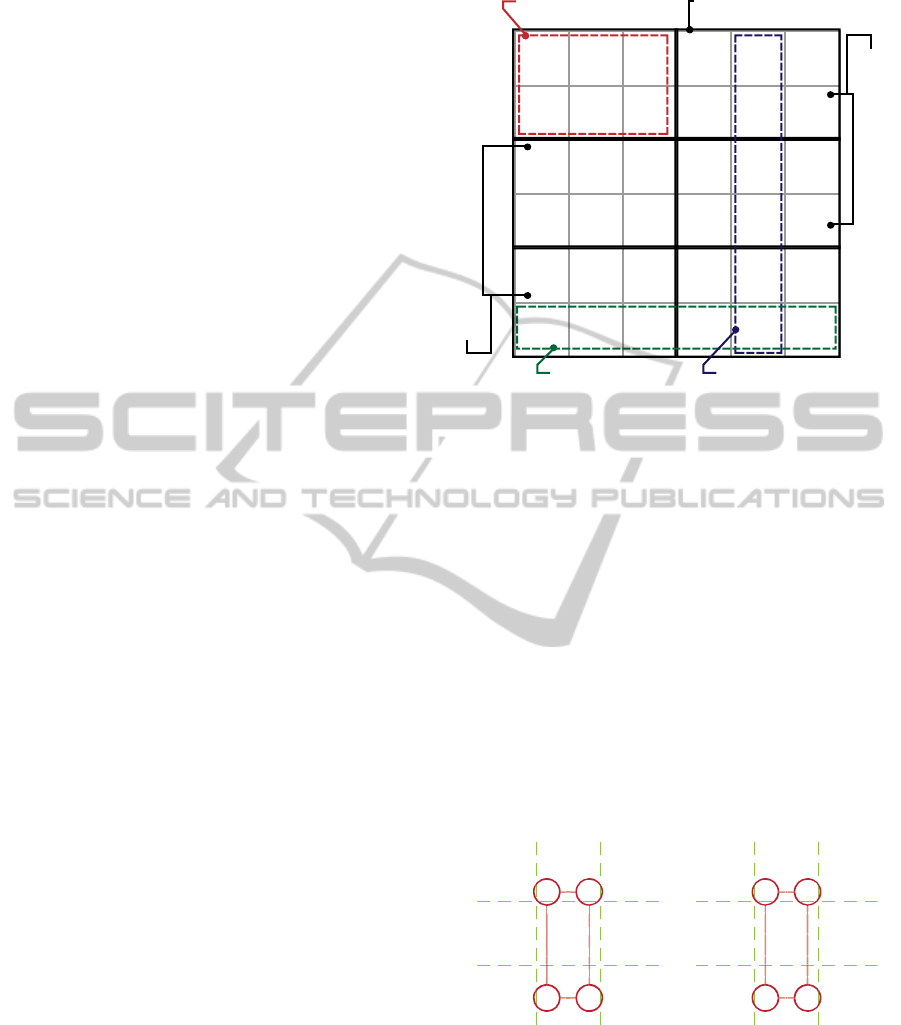
Figure 3: ‘Peers’ (light red) of [F,4] square (dark red).
In order to solve a Sudoku puzzle, blank squares
have to be completed with valid candidates until the
correct number is found; each square contains what
are called ‘Potential candidates’, or simply
‘Candidates’. The potential candidates are the
possible valid values of the set of integers: one to
nine, and each square has an exclusive set of
candidates while solving the puzzle. The set of valid
candidates can be described as follows (Crook,
2007; Edelkamp & Schrodl, 2012; Klingner &
Kanakia, 2013):
1,2,..,9
\
∪
∪
(2)
where denotes the valid candidates set of the
current square , and 1
|
|
. ,,
and are assigned values sets of ’s peers located
on row, column and sub-grid, respectively.
As previously mentioned, Sudoku solvers are
categorized to two main types, deductive and search
algorithms. Deductive algorithms are remarkably
slower and more difficult to develop because
immense coding effort is required (Norvig, 2010).
Each pattern requires a strategy to be recognized by
these algorithms, for instance, the ‘forbidden
rectangle’. A forbidden rectangle, as shown in
Figure 2, is a virtual rectangle that appears in the
Sudoku main grid, and all its corners have the same
candidates. This phenomenon prevents the puzzle
from having a unique solution. Thus, unless the
deductive algorithm is provided with sufficient tools
to manage this pattern (which is usually caused by
poor puzzle design), the algorithm ends without
solving the puzzle.
On the other hand, search algorithms, such as
BT, do not encounter problems when solving the
Sudoku set with forbidden rectangle. For example,
while solving the puzzle shown in Figure 2 (A), the
solver could assume that the correct answer for the
[C,4] square is the value five. This makes it
imperative for [C,6] to take the value eight, [H,4] to
also take eight, and [H,6] to take five because these
values are the only valid remaining ones.
Furthermore, the solver could make a different
decision by assuming that the correct answer for
[C,4] is eight. In this context, the assignment value
chain varies to fulfil the Sudoku rule, and the final
result is determined by the first assumption made.
This is attributed to the algorithm’s ability to
backtrack when a conflict occurs, and to attempt
other values.
In practice, the BT search algorithm goes into
iterative recursion calls called ‘labelling’ or
‘assignment’ process (Kumar, 1992), where one of
the candidates is placed in a square, while the others
are stored locally in case the chosen value fails to be
part of the solution. The algorithm continues
assigning values to new variables provided that the
values do not violate the Sudoku rule. However, if
they do, a conflict is declared and the algorithm
aborts the current labelling process in order to
backtrack. After reversing several steps (depending
on availability and the validity of the square
candidates), the algorithm tries other candidates until
the conflict is resolved. This is the basic principle of
backtracking, which is most likely to be a ‘trial and
error’ procedure (Eppstein, 2012; Moraglio et al.,
2006). In this paper, we consider this type of search
algorithm without involving any type of deductive
techniques to enhance efficiency.
BT is one of the most classical brute-force,
depth-first search algorithms (Kumar, 1992;
Moraglio et al., 2006) that guarantee finding a
solution for any Sudoku set (when there is one)
because all potential candidates are examined with
respect to the puzzle rule. Forward Checking (FC) is
considered an important improvement technique for
the BT algorithm, and it has the ability of
maintaining a list of valid values for each variable to
be examined. However, it does not follow a specific
strategy for selecting squares. Thus, the square
6
1
713
7
3
61
853
9 24856
5
4
2
12
3
4
5
6
7
8
9
A
B
C
D
E
F
G
H
I
ReorderingVariablesusing'ContributionNumber'StrategytoNeutralizeSudokuSets
327

selection (technically: node expansions) will take the
form of systematic order of selecting squares, for
instance, if the algorithm starts with the [A,1]
square; [A,2] is selected next unless it is occupied;
then [A,3] is selected, followed by [A,4], and so on,
until the last square [I,9]. Hence, if the algorithm
selects a square with many candidates at the
beginning, the probabilities of choosing incorrect
values are high. And, the solving process will have
to iterate through a wide search space before it
realizes the error, and the previously assigned values
are rendered useless.
Fortunately, the BT algorithm can exploit the
advantage of the MRV strategy. MRV is a “fail-
first” heuristic strategy that prioritizes and selects
squares based on the number of candidates that a
given square holds, i.e., the least candidates the
square has, the higher priority it receives (Russell &
Norvig, 2010). This does not prevent backtracking
from occurring, but is certain to reduce it.
Nonetheless, the MRV strategy still selects squares
randomly if there are two or more squares with the
same number of minimum values.
The CtN strategy is designed to select the most
promising square among those with the minimum
values in order to reduce the backtracking rate
further and to accelerate the solving process.
3 NEUTRALIZATION AND
SUDOKU NEUTRALIZED SET
People enjoy completing Sudoku puzzle squares
with numbers because they consider such puzzles as
mentally challenging activities and as ‘time killers’
(Crook, 2007). To such individuals, each square has a
solution and the puzzle is considered solved when
the last blank square is solved; however, algorithms
should not experience the same solving process.
Sudoku solvers reinforce the notion of maintaining
the algorithm engaged in searching process for as
long as there is at least one blank square without an
assigned value, and if there is any similarity between
them, it is their objective. As a result, the explored
squares to solve any Sudoku puzzle are at least equal
to the number of blank squares (variables) at the
initial configuration in the best-case scenario
(assuming no backtracking occurs).
The MRV strategy is attracted to squares with
one candidate because they guarantee that no
backtracking occurs given this selection process.
However, solving squares of this type does not
always improve the progress of solving the puzzle
given that the square value is not a candidate in any
of its peers. In this case, this square can be to be
treated as solved, and the algorithm can exclude it
from its search space. We call this a ‘Neutralized
Square’. If all remaining squares are neutralized, the
puzzle is considered solved; and so, the solving
process can. We call this configuration the
‘Neutralized Set’.
Figure 4: Neutralized Sudoku puzzle set.
The Sudoku puzzle shown in Figure 4 has 27
missing numbers that can be considered solved using
the neutralization concept. Search algorithms need
not be engaged in solving what it considers a
‘neutralized set’. With regard to the blank squares,
their values can be revealed through a validator to
confirm whether the only available solution is valid.
The neutralization concept covers two different
levels:
- Neutralized Square: a Sudoku blank square with
only one candidate, and all its peers are not
affected by solving the square. We consider any
engagement with this square as a redundant
iterative process for the solver.
- Neutralized Set: a Sudoku set where all the blank
squares are neutralized. In this case, the solver
has to declare the puzzle as ‘solved’, and all
searching activities are terminated.
A Sudoku neutralized configuration can be
mathematically described as follows:
(1)
where (Neutralization Number) is the result of
dividing (Total number of Blank Squares) over
(Total number of Remaining Candidates). The
puzzle is considered neutralized if 1. In other
words, if the total number of all remaining squares is
534
672
198
678
195
342
859
426
713
423
791
856
537
419
286
284
635
179
ICAART2015-InternationalConferenceonAgentsandArtificialIntelligence
328

equal to the total number of all potential candidates,
the puzzle is considered solved. Moreover,
neutralizing a solved puzzle is impossible because
both and are equal to zero, which results
in ∞.
Figure 5: (A) Algorithm lifecycle, (B) Algorithm lifecycle
with applications of the neutralization concept.
Hence, redefining the purpose the objective that
algorithms attempt to achieve is crucial; let i be the
initial configuration of a Sudoku puzzle to be solved
as illustrated in Figure 5. G is the goal of a search
algorithm delegated to solving the puzzle; the
algorithm requires iterative square explorations (in a
technical term: search recursion calls) to assign
values and achieve the goal, and these are denoted
R. Search algorithms such as BT with MRV
evaluate square candidates to identify the one to
select first, and then iterate through all the squares
recursively to assign them values in a labelling
process. The process continues to the last square,
unless a conflict occurs as mentioned earlier in this
paper. In this case, R is equal to the total number of
blank squares, plus any occurring backtracking. On
the contrary, the neutralization approach imposes a
sub-goal (denoted g) as shown in Figure 5 (B); the
search algorithm has to reach the sub-goal of
‘neutralizing the puzzle’ and decrease R by
increasing the number of neutralized squares
(denoted r).
In other words, the lifecycle of the BT search
algorithm with neutralization concept implemented
equals R (the number of blank squares occurring
backtracking) r (the neutralized squares). This
approach improves solving performance and
maintains resource consumption. The following
example illustrates a simple Sudoku puzzle: Figure 6
(A) shows a Sudoku set with 23 blank squares, most
of which have only one candidate as shown by the
grid in Figure 6 (B). By excluding the [B,7] and
[B,9] squares, selecting any square located in the last
six columns (4, 5, 6, 7, 8, 9) does not improve the
solving process because the squares have only one
candidate, and none of their peers consider their
values as potential candidates. In this case, MRV is
not the best strategy to use with the BT algorithm
because MRV cannot differentiate between the
competitive advantages of the puzzle squares, and
therefore, one of the squares will be selected
randomly; however, most of the squares are already
neutralized.
Evaluation of the Figure 6 (A) Sudoku set based
on neutralization principles reveals two optimal
squares located on [A,3] and ([C,1] or [B,7]);
solving the squares in this sequence leads to the
neutralization of all the remaining puzzle squares.
Thereafter, the puzzle is declared neutralized, the
algorithm terminates, and all resources reserved for
the solving process are released.
Finally, can function as an indicator of
Sudoku puzzle complexity because its value could
represent a reliable measurement equals to the ‘gap’
between the blank squares and their candidates, and
is limited to the following range:
1
9
1
(2)
If the value of a Sudoku set is close to one
and the set has many blank squares, the set difficulty
level can be considered easy, and vice versa.
4 CONTRIBUTION NUMBERS
The basic core of neutralization is to rely on altering
the algorithm objective from solving the problem to
neutralizing it; however, the manner in which the
existing Sudoku algorithms work does not help to
neutralize a puzzle. Any new strategy designed for
neutralizing Sudoku puzzles has to allow algorithms
to neutralize as many squares as possible per
assignment during the labelling process. The
strategy that we developed has the ability of
identifying the optimal square among those with the
minimum remaining values to escalate eliminating
other square candidates. Furthermore, our perception
towards optimality in the domain of solving Sudoku
relies on finding a square with the minimum number
of candidates and the maximum number of similar
candidates that exist among square peers. This is
because is reduced faster and neutralization is
accelerated. In other words, the optimal square
considers the following two criteria:
Number of potential candidates.
Ability to deduct candidates from square peers.
At first, the CtN strategy selects squares with
minimum remaining values, and then assesses them
(if there is more than one) by assigning weights
based on the criteria indicated above. The square
with the highest CtN is selected first as a new
frontier of the progressive labelling process. The
G
i
G
g
i
rR
R
(A)
(B)
ReorderingVariablesusing'ContributionNumber'StrategytoNeutralizeSudokuSets
329

weights produced by this strategy can be
mathematically described as follows:
∑∑
∈
|
|
|
|
(1)
Because the objective is to eliminate as many
candidates as possible per value assignment, the
process starts computing the Contribution Number
() of the current evaluated square by counting
similar candidates within the square blank peers to
determine the square that has the most influence on
the others. As previously mentioned, there are
number of peers for each square (see Section 2,
Equation 1), we need to visit all except those with
assigned values. In this case, (which denotes the
count number of the unassigned peers of the current
square) is equal to:
|
|
|
|
|
|
(2)
where
is a set of all assigned squares located on
the row of square,
is a set of all assigned
squares located on the column of square, and
is a set of all assigned squares located in the sub-grid
of square . Thus, by computing
(where is
always limited to1), the number of blank
peers of the current square is identified.
The next step is to select one of those blank
squares and iterate through all its candidates to
determine whether one is a member of the current
square candidate set
; if such is the case, the
counter is increased by one. The total counting of
similar candidates will be then divided over the size
of square’s candidate set
|
|
. This ensures the
squares with minimum number of candidates will
get higher weights. The following paragraphs
elaborate Equation (1) in detail.
To demonstrate the efficiency of the proposed
strategy, we consider solving the Sudoku set from
Figure 6 (A) using BT with FC technique, MRV,
and CtN strategies. All of them are subjected to the
sub-goal ‘Neutralization’. Starting with BT, the
algorithm selects frontiers in a systematic order. In
the worst-case scenario (as shown in
Figure 7 (A-1)),
the algorithm selects invalid values to be examined
at the beginning. This justifies backtracking because
wrong values are selected. As a result, the algorithm
must go through eight explored squares and three
backtrackings; the performance can be improved
slightly if the algorithm selects all the correct values
from the beginning. In this case, the results are five
explored squares without backtracking (see
Figure 7
(A-2)). Furthermore, the worst-case scenario for
MRV is not better than the worst-case scenario for
FC. MRV successfully avoids backtracking because
squares with minimum values are selected first.
However, this also prevents MRV from becoming
neutralized earlier (see
Figure 7 (B-1)). MRV results
in 17 explored squares, though no backtracking
occurs. On the other hand, MRV can perform
exactly as CtN if optimal squares are selected first.
However, the probabilities of that are rather low.
The results of the solving process are two explored
squares (see Figure 7 (B-2)).
The ability of the CtN strategy to identify the
most promising squares protects it from having
worst-case scenarios (at least, in this example).
Figure 6(C) shows the calculated CtN of the blank
squares from Figure 6(A). The [A,3] square from the
puzzle has only one candidate, just like the other
unassigned squares; however, solving it first leads to
a reduction in the total candidate average by
eliminating the value seven from [A,2] and [B,1].
Thus, by computing CtNs of the puzzle squares, the
[A,3] square receives the highest weight for
algorithm selection for the first iterative recursion of
the solving process. At the second recursion, both
[C,1] and [B,7] squares have one candidate, but
solving either eliminates the value four from [B,1].
This makes [C,1] and [B,7] valuable for choosing;
the calculated weights at the second recursion are
Figure 6: Easy Sudoku puzzle set with candidates and CtN weights within two recursions.
9..8..253
123456789
.83.95.1.
.15372689
12.76.3.5
.56483.2.
.94.51876
6.9.481.2
83172.5.4
.
A
B
C
D
E
F
G
H
I
42136798
.7,67.14...
123456789
7,4,2
..6..4.7
4........
..8..9.4.
7.....9.1
3..2.....
.7.5...3.
.....9.6.
5
A
B
C
D
E
F
G
H
I ........
.
-
1
.
63.11...
123456789
-
2
.
8..1..2.2
2........
..1..1.1.
2.....1.1
1..1.....
.2.1...1.
.....1.1.
1
A
B
C
D
E
F
G
H
I ........
.1..11...
123456789
-
2.5..1..2.1
2........
..1..1.1.
1.....1.1
1..1.....
.1.1...1.
.....1.1.
1
A
B
C
D
E
F
G
H
I ........
(A) Given Numbers (B) Potential Candidates (C) CtNs weights at the
first recursion
(D) CtNs weights at the
second recursion
ICAART2015-InternationalConferenceonAgentsandArtificialIntelligence
330

Figure 7: Search trees compression.
illustrated in Figure 6(D). The puzzle is declared
neutralized immediately following two square
assignments, and the algorithm is terminated at that
moment. It is noticeable that the CtN strategy
produces negative values, as seen in Figure 6(C) and
(D); this occurs because the remaining candidate
numbers for the squares with negative weights are
larger than some non-neutralized squares. The
strategy considers such squares undesirable choices
and multiplies them with -1 to ensure they are never
selected at this stage.
As part of our empirical experiments, we
developed the components, strategies, and core of
the search algorithm using the C# language to
evaluate strategy performance. The BT algorithm
and MRV strategy were adopted from a Python
program (Norvig, 2010) (but the deductive part
‘constraint propagation’ was excluded). The core of
the BT algorithm was developed as an independent
component and extensively shared for use by the
tested strategies and techniques to standardize the
algorithm performance.
5 RESULTS AND DISCUSSION
For the purpose of assessing the strategies, we
generated approximately 900 valid Sudoku puzzles
with three difficulty levels: easy, medium, and
difficult. The criteria for classifying Sudoku
difficulty levels were adopted from Sudoku Puzzles
Generating: from Easy to Evil (Jiang et al., 2009).
The results show that BT with FC requires more
iterative recursions because it continues to choose
incorrect squares with incorrect values when
following a systematic order for selecting squares.
The search algorithm uses a reasonable number of
iterative recursions to solve easy Sudoku sets, but
this number increases tremendously as the puzzles
become more difficult. However, MRV selects
squares based on their values (squares with
minimum candidates are solved first), which shows
great improvement on the number of explored
squares; this is caused by a significant reduction in
backtracking as the strategy targets squares with
minimum values. The CtN strategy shows an even
more disciplined behaviour for selecting squares
among those with fewer candidates, and the results
reflect a greater reduction in iterative recursions, in
particular for easy and medium difficulty sets.
However, difficult Sudoku puzzles represent a
challenge for the solver because squares with a
similar number of candidates are fewer than
expected. Sometimes, CtN acts exactly as MRV
when solving difficult Sudoku puzzles.
Nevertheless, the results show an improvement on
algorithm performance compared with MRV.
Tables
1 and 2 list the recursions required to solve the 900
different Sudoku sets, and the backtracking
occurrences during the solving process.
7
[A,2]
6
[A,2]
2
[B,1]
7
[A,3]
4
[A,6]
1
[A,5]
4
[B,1]
0
[A,3]
0
[B,7]
6
[B,4]
Su b
-
Goal
6
[A,2]
2
[B,1]
7
[A,3]
4
[A,6]
1
[A,5]
Su b
-
Go al
(A-1) FC (Explored square: 8, Backt racking:3 )
(Worst-case scenario)
(A-2) FC (Explored square: 5, Backtracking:0 )
(Best-case scenario)
1
[A,5]
4
[A,6]
6
[B,4]
3
[F,1]
9
[E,7]
6
[H,8]
9
[D,6]
5
[G,4]
2
[F,4]
4
[D,8]
7
[B,9]
4
[C,1]
1
[E,9]
7
[A,3]
3
[G,8]
9
[H,6]
5
[i,1]
Su b
-
Goal
(B-1) MRV (Explored square: 17, Backtracking:0 )
(Worst-case scenario)
7
[A,3]
4
[C,1]
Su b
-
Goal
(B-2) MRV (Explored square: 2, Backtracking:0 )
(Best-case scenario)
7
[A,3]
4
[B,7]
Su b
-
Goal
(C) CtN (Explored-square: 2, Backt racking:0 )
ReorderingVariablesusing'ContributionNumber'StrategytoNeutralizeSudokuSets
331

Accordingly, CtN requires exploring nearly 1/3
fewer squares than MRV, but not for difficult
puzzles. The number of squares with minimum
remaining candidates is limited for difficult sets,
which means that the strategy has fewer squares to
evaluate. This leads CtN to behave similarly to
MRV at that difficulty level. As the solving process
advances, the number of squares with the same
minimum number of candidate increases, and their
influence on their peers is more distinct.
Table 1: The average of recursions required to neutralize
900 Sudoku sets.
Strategies/
techniques
Difficultylevel
Easy
Clues:41‐53
Medium
Clues:30‐40
Difficult
Clues:22‐29
FC 45 394 84,594
MRV 33 48 215
CtN 10 26 171
Table 2: The average of backtracking that occurs when
solving Table 1 Sudoku sets.
Strategies/
techniques
Difficultylevel
Easy
Clues:41‐53
Medium
Clues:30‐40
Difficult
Clues:22‐29
FC 12 341 84,539
MRV 1 4 161
CtN 1 1 132
Overall, the achievement to be highlighted is the
ability of the BT algorithm that uses the CtN
strategy to neutralize Sudoku puzzles with minimum
iterative recursions. Figure 8 reflects the results of
neutralizing 900 Sudoku puzzle using MRV and
CtN. The figure shows the efficiency of CtN to
neutralize easy and medium Sudoku sets; FC is
excluded because its values cannot be represented on
the chart as its results are extremely greater than the
graph scale.
6 CONCLUSIONS
In this paper, we presented a new strategy for
Sudoku algorithms that can accelerate the solving
process, reduce the number of required explored
squares, and minimize the number of backtracking
occurrences. The puzzle is declared ‘neutralized’
once the sub-goal is achieved. Moreover, the
concept of achieving a sub-goal relies on re-ordering
and prioritizing the puzzle's blank squares as the
solving process progresses based on the influences
on their pairs and the number of candidates. In order
to do so, an evaluation method assesses all existing
blank squares in a puzzle and assigns their weights;
we called this strategy the Contribution Number
(CtN) strategy.
ACKNOWLEDGEMENTS
We gratefully acknowledge the support provided by
Universiti Teknologi MARA (UiTM) and the
Japanese Student Service Organization (JASSO).
This work was supported by JSPS KAKENHI Grant
Number 23300056.
Figure 8: Performance of neutralizing 900 Sudoku puzzles using MRV and CtN.
0
50
403020 50
Gi v en Nu m b er
s
100
150
200
Iterative
Re c u r s i o n s
250
453525
MRV Recursions
MRV Backtraki ng
CtN Recursions
Ct N Back tr ak i n g
Ea sy
Medium
Di cult
Sudoku di cul ty levels:
ICAART2015-InternationalConferenceonAgentsandArtificialIntelligence
332

REFERENCES
Aaronson, L. 2006. Sudoku Science. Spectrum, IEEE,
43(2), 16–17. doi:10.1111/birt.12116.
Crook, J. F. 2007. A Pencil-and-Paper Algorithm for
Solving Sudoku Puzzles, 56(4), 460–468.
Edelkamp, S., & Schrodl, S. 2012. Heuristic Search:
Theory and Applications, (pp. 574–631). Waltham:
Elsevier Inc.
Eppstein, D. 2012. Solving Single-digit Sudoku
Subproblems. In Kranakis, E., Krizanc, D., & Luccio,
F. Eds., Fun with Algorithms, 7288, 142–153.
Springer Berlin Heidelberg..
Ercsey-Ravasz, M., & Toroczkai, Z. 2012. The Chaos
within Sudoku. Scientific Reports, 2, 725.
doi:10.1038/srep00725.
Jiang, B., Xue, Y., Li, Y., & Yan, G. 2009. Sudoku
Puzzles Generating : from Easy to Evil. Chinese
Journal of Mathematics in Practice and Theory, 39,
1–7.
Jilg, J., & Carter, J. 2009. Sudoku Evolution, April 1984,
173–185.
Klingner, J., & Kanakia, A. 2013. Methods for Solving
Sudoku Puzzles, 1–10.
Kumar, V. 1992. Algorithms for Constraint Satisfaction
Problems: A Survey. AI Magazine, 13(1), 32–44.
Mcguire, G., Tugemann, B., & Civario, G. 2014. There is
no 16-Clue Sudoku : Solving the Sudoku Minimum
Number of Clues Problem via Hitting Set
Enumeration. Experimental Mathematics, 23(2), 190–
217.
Moraglio, A., Togelius, J., & Lucas, S. 2006, Product
Geometric Crossover for the Sudoku Puzzle. IEEE
International Conference on Evolutionary
Computation, 470–476. doi:10.1109/CEC.2006.
1688347.
Norvig, P. 2010. Solving Every Sudoku Puzzle, Retrieved
July 16, 2014, from http://www.norvig.com/
sudoku.html.
Russell, S., & Norvig, P. 2010. Artificial Intelligence: A
Modern Approach (Third Ed., pp. 206–202). Pearson.
ReorderingVariablesusing'ContributionNumber'StrategytoNeutralizeSudokuSets
333
