Speaker Identification with Short Sequences of Speech Frames
Giorgio Biagetti, Paolo Crippa, Alessandro Curzi, Simone Orcioni and Claudio Turchetti
DII – Dipartimento di Ingegneria dell’Informazione, Universit`a Politecnica delle Marche,
Via Brecce Bianche 12, I-60131 Ancona, Italy
Keywords:
Speaker Identification, Speaker Recognition, Classification, Speech, Speech Frames, Short Sequences, DKLT,
GMM, EM Algorithm, MFCC, Cepstral Analysis, Feature Extraction, Digitized Voice Samples.
Abstract:
In biometric person identification systems, speaker identification plays a crucial role as the voice is the more
natural signal to produce and the simplest to acquire. Mel frequency cepstral coefficients (MFCCs) have
been widely adopted for decades in speech processing to capture the speech-specific characteristics with a
reduced dimensionality. However, although their ability to de-correlate the vocal source and the vocal tract
filter make them suitable for speech recognition, they show up some drawbacks in speaker recognition. This
paper presents an experimental evaluation showing that reducing the dimension of features by using the dis-
crete Karhunen-Love transform (DKLT), guarantees better performance with respect to conventional MFCC
features. In particular with short sequences of speech frames, that is with utterance duration of less than 1 s,
the performance of truncated DKLT representation are always better than MFCC.
1 INTRODUCTION
Biometric person identification systems based on hu-
man speech are increasingly being used as a means
for the recognition of people. Among the most popu-
lar measurements for identification, voice is the more
natural signal to produce and the simplest to acquire,
as the telephone system provides an ubiquitous net-
work of sensors for delivering the speech signal (Jain
et al., 2004; Bhardwaj et al., 2013). Typical ap-
plications are access control, telephone services for
transaction authorization in place of password or PIN,
speaker diarization.
Speaker recognition is the key research area in de-
veloping speaker recognition technologies which uti-
lize speech to recognize, identify or verify individ-
uals (Togneri and Pullella, 2011; Kinnunen and Li,
2010; Reynolds, 2002) and can be categorized into
two fundamental modes of operations: identification
and verification. In identification systems, the issue
is to detect which speaker from a given pool the un-
known speech is derived from, while in verification
systems the speech of the unknown person is com-
pared against both the claimed identity and against all
other speakers (the imposter or background model)
(Gish and Schmidt, 1994; Campbell, 1997; Bimbot
et al., 2004). Both tasks fall into the general prob-
lem of statistical pattern recognition, in which a given
pattern is to be assigned to one of a set of differ-
ent categories (Jain et al., 2000). From this point of
view, the main difference between speaker identifica-
tion and speaker verification is that in the first one
the classification is based on a set of S models (one
for each speaker), while, in the second case, a total of
two models (one for the hypothesizedspeaker and one
for the background model), have to be derived during
training.
This paper addresses the problem of speaker iden-
tification with short sequences of speech frames, that
is with utterance duration of less than 1 s. In partic-
ular, as this is a very severe test for speaker identi-
fication, we want to investigate for feature represen-
tations of voice sample that guarantees the best per-
formance in terms of classification accuracy. This
is motivated by the fact that although Mel frequency
cepstral coefficients(MFCCs) havedemonstrated par-
ticularly suitable for speech recognition, they present
some drawbacks in speaker recognition. In particu-
lar, the speaker variability due to pitch mismatch, that
is a specific characteristic that distinguishes different
speakers, is greatly mitigated by smoothing property
of the MFCC filter bank (Zilca et al., 2006). Besides,
with reference to the accuracy of dimensionality re-
duction techniques and their application to speaker
identification, the MFCC linear transform does not
guarantees any convergence properties as the dimen-
sion of subspace tends to the dimension of the frame.
It is well known that among linear transforms that
178
Biagetti G., Crippa P., Curzi A., Orcioni S. and Turchetti C..
Speaker Identification with Short Sequences of Speech Frames.
DOI: 10.5220/0005191701780185
In Proceedings of the International Conference on Pattern Recognition Applications and Methods (ICPRAM-2015), pages 178-185
ISBN: 978-989-758-077-2
Copyright
c
 2015 SCITEPRESS (Science and Technology Publications, Lda.)

can be used for feature extraction and dimensional-
ity reduction, the best known linear feature extractor
is the discrete Karhunen-Love transform (DKLT) ex-
pansion. In addition, as robust speaker recognition
remains an important problem in speaker identifica-
tion (Zhao et al., 2012; Maina and Walsh, 2011; Zhao
et al., 2014; McLaughlin et al., 2013; Sadjadi and
Hansen, 2014), in a recent paper (Patra and Acharya,
2011) it has been shown that principal component
analysis (PCA) transformation minimizes the effect
of noise and improves the speaker identification rate
as compared to the conventional MFCC features.
In this work we want to show that the truncated
version of DKLT, that is with a subset of components,
exhibits good performance in terms of classification
accuracy, without affecting speaker variability as in
MFCCs filtering approach occurs. In a comparison
with standard approach, experimental results clearly
show that truncated DKLT behaves better than MFCC
features.
2 SINGLE FRAME SPEAKER
IDENTIFICATION
2.1 Bayesian Classification
Let us refer to a frame y[n], n = 0,..., N − 1, rep-
resenting the power spectrum of speech signal, ex-
tracted from the time domain waveform of the utter-
ance under consideration, through a pre-processing
algorithm including pre-emphasis, framing and log-
spectrum. Typical duration values for frames ranges
from 20 ms to 30 ms (usually 25 ms) and a frame is
generated every 10 ms (thus consecutive25 ms frames
generated every 10 ms will overlap by 15 ms).
The problem of classification is in general stated
as: Given a set W of tagged data (training set), such
that each of them is known to belong to one of S
classes, and a set Z of data (testing set) to be clas-
sified, determine a decision rule establishing which
class an element y ∈ Z belongs to.
Thus in the context of spectrum identification we
assume that the speech from each known, verified
speaker, for all speakers that need to be identified, is
acquired and divided in two sets, W for training and
Z for testing.
For Bayesian speaker identification, a group of S
speakers is represented by the pdf’s
p
s
(y) = p(y | θ
s
) , s = 1,··· ,S (1)
where θ
s
are the parameters to be estimated during
training, y ∈ W . Thus we can define the vector,
p = [p
1
(y),··· , p
S
(y)]
T
. (2)
The objective of classification is to find the speaker
model θ
s
which has the maximum a posteriori proba-
bility for a given frame y ∈ Z. Formally:
ˆs(y) = argmax
1≤s≤S
{p
r
(θ
s
|y)} = argmax
1≤s≤S

p(y|θ
s
)p
r
(θ
s
)
p(y)

(3)
Assuming equally likely speakers (i.e. p
r
(θ
s
) =
1/S ) and noting that p(y) is the same for all speakers
models, the Bayesian classification is equivalent to
ˆs(y) = argmax
1≤s≤S
{p(y|θ
s
)} , (4)
or in a more compact form to
ˆs(y) = arg{kpk
∞
} , (5)
where
kpk
∞
= max
1≤s≤S
{p
s
(y)} (6)
is the maximum or infinity norm. Thus speaker
Bayesian identification reduces to solving the prob-
lem stated by (5).
2.2 GMM Model Estimation
The most generic statistical speaker modeling one
can adopt is the Gaussian mixture model (GMM)
(Reynolds and Rose, 1995). The GMM for the single
speaker, is a weighted sum of F components densities
and given by the equation
p(y|θ) =
F
∑
i=1
α
i
N (y | µ
i
,C
i
) (7)
where α
i
, i = 1,... , F are the mixing weights, and
N (y|µ
i
,C
i
) =
(2π)
−
N
2
p
|C
i
|
exp
(
−
(y−µ
i
)
T
C
−1
i
(y−µ
i
)
2
)
(8)
represents the density of a Gaussian distribution with
mean µ
i
and covariance matrix C
i
. It is worth noting
that α
i
must satisfy 0 ≤ α
i
≤ 1 and
∑
F
i=1
α
i
= 1. θ ( the
index s is omitted for the sake of notation simplicity)
is the set of parameters needed to specify the Gaussian
mixture, defined as
θ = {α
1
,µ
1
,C
1
,... ,α
F
,µ
F
,C
F
} . (9)
As the maximum likelihood (ML) estimate of θ,
ˆ
θ
ML
= argmax
θ
{log p(W | θ)} (10)
with training data W is difficult to find analytically
due to the log of the sum in (10), the usual choice
for solving ML estimate of the mixture parameters is
the expectation maximization (EM) algorithm. This
algorithm is based on a set H = {h
(1)
,... ,h
(L)
} of
SpeakerIdentificationwithShortSequencesofSpeechFrames
179

L labels associated with the L observations, each la-
bel being a binary vector h
(ℓ)
= [h
(ℓ)
1
, ... , h
(ℓ)
F
], where
h
(ℓ)
i
= 1 and h
(ℓ)
l
= 0 for all l 6= i, means that the vector
y
(ℓ)
∈ W was generated by the i-th Gaussian compo-
nent N (y|µ
i
,C
i
). The EM algorithm is based on the
interpretation of W as incomplete data and H as the
missing part of the complete data X = {W ,H }. The
complete data log-likelihood, i.e. the log-likelihood
of X as though H was observed, is
log[p(W , H |θ)] =
L
∑
ℓ=1
F
∑
i=1
h
(ℓ)
i
log
h
α
i
N (y
(ℓ)
|µ
i
,C
i
)
i
.
(11)
In general the EM algorithm computes a sequence
of parameter estimates

ˆ
θ(p) , p = 0,1,...

by itera-
tively performing two steps:
• Expectation Step: computes the expected value of
the complete log-likelihood, given the training set
W and the current parameter estimate
ˆ
θ(p). The
result is the so-called auxiliary function
Q

θ|
ˆ
θ(p)

= E

log[p(W , H |θ)]|W ,
ˆ
θ(p)

.
(12)
• Maximization Step: update the parameter estimate
ˆ
θ(p+ 1) = argmax
θ

Q

θ|
ˆ
θ(p)

(13)
by maximizing the Q-function.
Recently, Figueiredo et al. (Figueiredo and Jain,
2002) suggested an unsupervised algorithm for learn-
ing a finite mixture model from multivariate data, that
overcomes the main lacks of the standard EM ap-
proach, i.e. sensitiveness to initialization and selec-
tion of number F of components. This algorithm in-
tegrates both model estimation and component selec-
tion, i.e. the ability of choosing the best number of
mixture components F according to a predefined min-
imization criterion, in a single framework. In particu-
lar, it is able to perform an automatic component an-
nihilation directly within the maximization step of the
EM iterations.
2.3 The Problem of Dimensionality
Reduction
For usually 8 kHz (16 kHz) bandwidth speech the
vector y has a dimension N = 128 (256). Although
the Figueiredo’s EM algorithm behaves well with
multivariate random vectors, a too large amount of
training data would be necessary to estimate the pdf
p(y | θ
s
) and, in any case, with such a dimension the
estimation problem is impractical.
2.3.1 DKLT Truncation
In order to face the problem of dimensionality, the
usual choice is to reduce y to a vector k
M
of lower
dimension by a linear non-invertible transform H (a
rectangular matrix) such that
k
M
= H y , (14)
y ∈ R
N
, k
M
∈ R
M
, H ∈ R
M× N
, and M ≪ N. The vec-
tor k
M
represents the so-called feature-vector belong-
ing to an appropriate subspace of dimensionality M.
It is well known that, among the allowable linear
transforms H : R
N
→ R
M
, the DKLT truncated to M <
N orthonormal basis functions, is the one that ensures
the minimum mean square error (Therrien, 1992).
More formally, let us consider the vector y[n],
n = 0,... , N − 1, as an observation of the N × 1 real
random vector y = [y
1
,... ,y
N
]
T
whose autocorrela-
tion function is given by R
yy
= E

yy
T

, where the
symbol E{·} denotes the expectation.
Once R
yy
is estimated, an orthonormal set
{φ
1
,... , φ
N
}, can be derivedas a solution of the eigen-
vector equations
R
yy
= ΦΛΦ
T
(15)
where Λ = diag(λ
1
,... ,λ
N
), Φ = [φ
1
,... ,φ
N
] ∈
R
N×N
.
The DKLT of y is defined by the couple of equa-
tions
k = Φ
T
y , (16)
y = Φ k , (17)
where k = [k
1
,... ,k
N
]
T
is the transformed random
vector (Fukunaga, 1990).
In order to evaluate the effect of truncation on
DKLT, let us rewrite (17) as:
y = Φ k = Φ
M
k
M
+ Φ
η
k
η
= x
M
+ η
y
, (18)
where Φ = [Φ
M
, Φ
η
], being Φ
M
= [φ
1
,... ,φ
M
] ∈
R
N×M
, k
M
∈ R
M
, and (16) as:

k
M
k
η

=

Φ
T
M
Φ
T
η

y . (19)
In (18)
x
M
= Φ
M
k
M
, (20)
is the truncated expansion, and
η
y
= Φ
η
k
η
, (21)
is the error or residual. The truncation is equivalent to
the approximations
y ≈ x
M
, k ≈ k
T
=

k
M
0

, (22)
ICPRAM2015-InternationalConferenceonPatternRecognitionApplicationsandMethods
180

thus, as k
M
is given by
k
M
= Φ
T
M
y , (23)
comparing (23) with (14) yields H = Φ
T
M
. This is
equivalent to the PCA that extracts the most impor-
tant features of data.
It can be shown (Therrien, 1992) that the mini-
mum mean square error E
M
= E

η
T
y
η
y

, subject to
the constraints φ
T
i
φ
i
= 1, i = M+ 1,... , N, is given by
E
M
= E

ky− x
M
k
2

= E

(y− x
M
)
T
(y− x
M
)

=
N
∑
i=M+1
λ
i
, (24)
where λ
i
is the eigenvalue corresponding to the eigen-
vector φ
i
. Once the λ
i
are arranged in decreasing or-
der, the error E
M
decreases monotonically as the in-
dex M increases towards N.
2.4 Bayesian Classification by
Truncation
Given a group of S speakers, the pdf’s
p
s
(k
T
) = p(k
T
| θ
s
) , s = 1,··· ,S (25)
can be derived, where k
T
is the truncation of k, and
consequently also the vector
˜p = [p
1
(k
T
),·· · , p
S
(k
T
)]
T
, (26)
which represents an approximation of the vector p in
(2), is defined. Thus (5) becomes:
ˆs(y) = arg{k˜pk
∞
} . (27)
However, since
k˜pk
∞
= max
1≤s≤S
{p
s
(k
T
)} , (28)
and from (22) we have
p
s
(k
T
) = p
s
(k
M
) δ(k
η
) , (29)
it results
k˜pk
∞
= max
1≤s≤S
{p
s
(k
M
) δ(k
η
)} = max
1≤s≤S
{p
s
(k
M
)} .
(30)
As you can see comparing (30) with (6), the
dimensionality of classification problem is reduced
from N to M, with M < N.
3 MULTI-FRAME SPEAKER
IDENTIFICATION
The accuracy of speaker identification can be consid-
erably improved using a sequence of frames instead
of a single frame alone. To this end let us refer to
a sequence of frames defined as Y = {y
(1)
,... , y
(V)
}
where y
(v)
represents the v-th frame. Using (27) and
(30) we can determine the class each frame y
(v)
be-
longs to. Thus the S sets
Z
s
=
n
y
(v)
| y
(v)
belongs to class S
o
, s = 1,...S ,
(31)
are univocally determined.
Given Y, we define the score for each class s as:
r
s
(Y) = card{Z
s
} , (32)
where the operator card{·} (cardinality) extracts the
number of elements belonging to Z
s
. Finally the
multi-frame speaker identification is based on:
ˆs(Y) = argmax
1≤s≤S
{r
s
(Y)} . (33)
4 EXPERIMENTAL RESULTS
4.1 Data Base
The experiments were carried out on a large identi-
fication corpus based on the audio recordings of five
different speakers, two females (A, B) and three males
(C, D, E) as reported in Table 1. The material was
originally extracted from five freely available Italian
audiobooks. All recordings are mono, 8 kilosamples
per second, 16 bit, particularly suitable for telephone
applications.
Figure 1 shows the block diagram of the proposed
front-end employed for feature extraction. At the in-
put of the processing chain a voice activity detection
block drops all non speech segments from the input
audio records, exploiting the energy acceleration as-
sociated with voice onset. The signal is then divided
into overlapping frames of 25 ms (200 samples), with
a frame shift of 10 ms (80 samples). Hence buffer-
ing is required for storing overlapping regions among
frames. Besides, before computing the DKLT fea-
tures, each frame is cleaned up by a noise reduc-
tion block based on the Wiener filter. Further en-
hancements are then performed by a SNR-dependent
waveform processing phase, that weights the input
noise-reduced frame according to the positions of its
smoothed instant energy contour maxima. It is worth
noting that noise reduction introduces an overall la-
tency of 30 ms (3 frames) due to its algorithm requir-
ing internal buffering.
The consistency of DBT database in terms of
number of frames used for each speaker is reported
in Table 2.
SpeakerIdentificationwithShortSequencesofSpeechFrames
181

Table 1: Recordings used for the creation of the identification corpus. Source: liber liber (http://www.liberliber.it/). The
material was used both for training and testing purposes.
Speaker Gender Audiobook Chapter Duration [s]
A F “Il giornalino di Gianburrasca” by L. Bertelli I 761
B F “I promessi Sposi” by A. Manzoni I 2593
C M “Fu Mattia Pascal” by L. Pirandello I 251
D M “Le tigri di Mompracem” by E. Salgari I 838
E M “I Malavoglia” by G. Verga I 1162
Framing
and
buering
Noise
reduction
stage
<>d
feature
extraction
SNR-dep.
waveform
processing
Voice
activity
detection
Figure 1: The proposed front-end for feature extraction.
Table 2: Consistency of the databases used for experimental evaluation.
Database DBT DB1 (80:20) DB2 (50:50) DB3 (20:80)
Speaker train test train test train test
A 58903 47122 11781 29451 29452 11780 47123
B 195591 156472 39119 97795 97796 39118 156473
C 18867 15093 3774 9431 9434 3773 15094
D 63713 50970 12743 31856 31857 12742 50971
E 91253 73002 18251 45626 45627 18250 73003
Total 428327 342659 85668 214161 214166 85663 342664
From DBT the databases DB1, DB2, and DB3,
with different percentage consistency of training and
testing subsets, have been derived. More in detail for
generating the DB2 database we divided the full DBT
database in two datasets containingfor each of the five
speakers the same proportionof speech frames chosen
by considering the first part of them (50%) for train-
ing (model evaluation) and the second part (50%) for
testing (performance evaluation) purposes. In a sim-
ilar manner, the DB1 and DB3 databases have been
generated by assigning to the testing set / training set
ratio the values of 80% / 20% and 20% / 80% respec-
tively.
4.2 Speaker Identification with
Truncated DKLT
Several experiments were performed by varying the
number of DKLT components retained in the GMM
model, with the three different databases in order to
evaluate the effect of training data amount on the clas-
sification results. An optimum value of 12 DKLT
components has been chosen for the GMM model.
With the frames belonging to the testing sets, we
ran our classifier and counted the number of occur-
rences of each recognized type, so as to obtain a con-
fusion matrix for every speaker identification experi-
ment. The resulting confusion matrices are reported
in Table 3 for the single-frame, and in Table 4 for
the multi-frame (V = 100) speaker identification to
illustrate in detail the performance of single-frame
identification as well as the improvement of the ac-
curacy when 100 consecutive frames (corresponding
to a speech sequence of 1s) have been used for the
speaker classification.
To gain some insight on the performance of the
method, the standard set of performance indices for
classification was also extracted from the confusion
matrices. To this end we computed the sensitivity,
specificity, precision and accuracy, defined as
sensitivity = TP/(TP+ FN) (34)
specificity = TN/(TN+ FP) (35)
precision = TP/(TP+ FP) (36)
accuracy = (TP+ TN)/(TP+ TN+ FP+ FN) (37)
where TP are the true positives(the diagonal elements
ICPRAM2015-InternationalConferenceonPatternRecognitionApplicationsandMethods
182

Table 3: Single-frame confusion matrices, for the different
DB1, DB2, and DB3 databases, obtained by considering 12
DKLT components.
Recognized
Input A B C D E
DB1 (80:20)
A 9885 688 349 312 547
B 1927 35226 570 720 676
C 200 100 2313 573 588
D 812 384 2113 6831 2603
E 1165 429 2443 2648 11566
DB2 (50:50)
A 23729 2166 1138 823 1596
B 4027 89214 1401 1810 1344
C 427 270 5444 2185 1108
D 1925 1151 5590 17199 5992
E 2919 1232 6265 8400 26811
DB3 (20:80)
A 36552 5135 1682 1395 2359
B 6104 143531 2018 2973 1847
C 708 557 9132 2671 2026
D 3364 2183 10957 24372 10095
E 6186 2587 11127 12613 40490
of the confusion matrix), FN the false negatives (the
sum of the other elements on the same row of the con-
fusion matrix), FP the false positives (the sum of the
other elements on the same column of the confusion
matrix), and TN the true negatives(the sum of the ele-
ments on the other rows and columns of the confusion
matrix). Additionally we considered the overall sen-
sitivity, also named correct identification rate (CIR)
by some authors, defined as the ratio of the sum of the
diagonal elements (true positives) respect to the sum
of all the elements of the confusion matrix.
The results for 12 DKLT components are reported
in Table 5 for the multi-frame (V = 100) speaker
identification. Also in this case the effect of the
database consistency has been investigated. The over-
all sensitivity obtained in the single frame identifi-
cation is of 76.83%, 75.83%, and 74.15% for DB1,
DB2, and DB3 databases, respectively. Significantly
greater values have been obtained in the multi-frame
(sequence of V = 100 consecutive frames) case i.e.
99.65%, 98.55%, and 95.71% for DB1, DB2, and
DB3 databases, respectively.
Table 4: Multi-frame (V = 100) confusion matrices, for the
different DB1, DB2, and DB3 databases, obtained by con-
sidering 12 DKLT components.
Recognized
Input A B C D E
DB1 (80:20)
A 117 0 0 0 0
B 0 391 0 0 0
C 0 0 36 0 1
D 0 0 1 125 1
E 0 0 0 0 182
DB2 (50:50)
A 294 0 0 0 0
B 0 977 0 0 0
C 1 0 89 4 0
D 3 0 12 301 2
E 4 0 1 4 447
DB3 (20:80)
A 471 0 0 0 0
B 0 1564 0 0 0
C 0 0 148 1 1
D 11 0 31 436 31
E 42 0 10 20 658
To show the effect of the sequence length on the
speaker identification, Figs. 2 and 3 depict the sen-
sitivity as a function of the number V of the frames
for two different numbers of DKLT components M =
20 and 15, respectively, retained in the GMM model,
using the DB1 database.
4.3 Comparison with MFCC Model
To investigate the relative performance of our method
with the state of the art, we conducted for compari-
son some experiments using MFCC features. In this
case, 13 MFCC features have been considered and
the performance for all the databases has been re-
ported in Table 6 where sequences of 100 frames have
been considered for identification purposes. Addi-
tionally, the overall sensitivity obtained in this case is
of 93.33%, 94.81%, and 93.52% for DB1, DB2, and
DB3 databases, respectively. Comparing these results
with those of our method with 12 DKLT components
and 100 frames, it is evident that our method behaves
better than the MFCC-based one.
In particular, with reference to a sequence of V =
SpeakerIdentificationwithShortSequencesofSpeechFrames
183

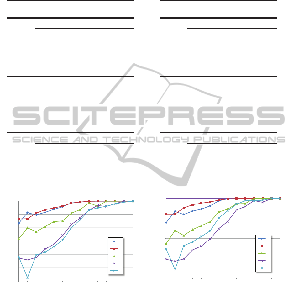
Table 5: Truncated DKLT performance analysis for the dif-
ferent databases (V = 100 frames, 12 DKLT components).
Speaker Sens. Spec. Prec. Acc.
(%) (%) (%) (%)
DB1 (80:20)
A 100.00 100.00 100.00 100.00
B 100.00 100.00 100.00 100.00
C 97.30 99.88 97.30 99.77
D 98.43 100.00 100.00 99.77
E 100.00 99.70 98.91 99.77
DB2 (50:50)
A 100.00 99.57 97.35 99.63
B 100.00 100.00 100.00 100.00
C 94.68 99.36 87.25 99.16
D 94.65 99.56 97.41 98.83
E 98.03 99.88 99.55 99.49
DB3 (20:80)
A 100.00 98.21 89.89 98.45
B 100.00 100.00 100.00 100.00
C 98.67 98.75 78.31 98.74
D 85.66 99.28 95.40 97.25
E 90.14 98.81 95.36 96.96
40
50
60
70
80
90
100
1 2 3 5 7 10 20 30 50 70 100 120 150 200
Sensitivity [%]
Sequence Length [frames]
A
B
C
D
E
Figure 2: Classifier performance as a function of sequence
length, with 20 DKLT components, using DB1 database.
100 frames, Tables 5 and 6 clearly show that all the
performance indices for truncated DKLT are better
than those for MFCC-based classifier. Similar results
are obtained by varying the sequence length, as Fig. 4
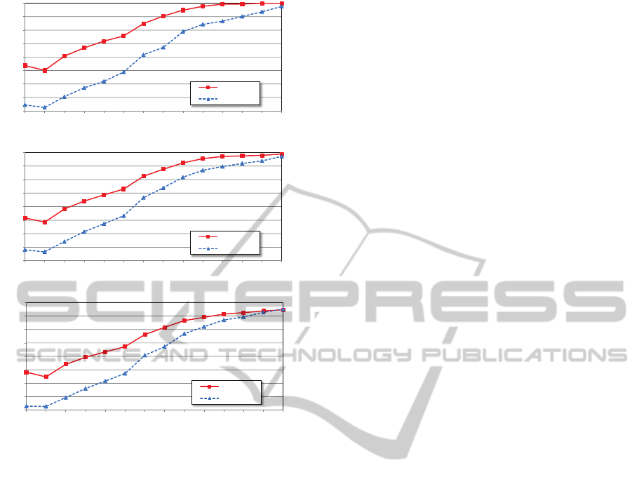
points-out.
In order to better compare the two methods, sev-
eral additional experiments were carried out. Fig. 4
reports, for a more intuitive comparison, the over-
Table 6: MFCC performance analysis for the different
databases (V = 100 frames).
Speaker Sens. Spec. Prec. Acc.
(%) (%) (%) (%)
DB1 (80:20)
A 100.00 96.34 81.25 96.84
B 93.35 99.78 99.73 96.84
C 94.59 98.65 76.09 98.48
D 94.49 98.35 90.91 97.78
E 87.91 99.11 96.39 96.72
DB2 (50:50)
A 100.00 97.62 86.98 97.94
B 96.72 99.83 99.79 98.41
C 85.11 99.56 89.89 98.92
D 96.23 97.69 87.93 97.48
E 88.38 99.17 96.64 96.87
DB3 (20:80)
A 99.36 98.68 92.31 98.77
B 98.02 99.57 99.48 98.86
C 84.67 98.78 76.05 98.16
D 92.14 96.54 82.28 95.88
E 82.88 98.74 94.68 95.36
40
50
60
70
80
90
100
1 2 3 5 7 10 20 30 50 70 100 120 150 200
Sensitivity [%]
Sequence Length [frames]
A
B
C
D
E
Figure 3: Classifier performance as a function of sequence
length, with 15 DKLT components, using DB1 database.
all sensitivity as a function of speech sequence and
database consistency. As you can see, and in particu-
lar for short sequences, the truncated DKLT behaves
always better than the MFCC-based counterpart.
ICPRAM2015-InternationalConferenceonPatternRecognitionApplicationsandMethods
184

60
65
70
75
80
85
90
95
100
1 2 3 5 7 10 20 30 50 70 100 120 150 200
Sensitivity [%]
Sequence Length [frames]
dim12 (DB1)
MFCC (DB1)
(a)
60
65
70
75
80
85
90
95
100
1 2 3 5 7 10 20 30 50 70 100 120 150 200
Sensitivity [%]
Sequence Length [frames]
dim12 (DB2)
MFCC (DB2)
(b)
60
65
70
75
80
85
90
95
100
1 2 3 5 7 10 20 30 50 70 100 120 150 200
Sensitivity [%]
Sequence Length [frames]
dim12 (DB3)
MFCC (DB3)
(c)
Figure 4: Overall sensitivity of MFCC features and trun-
cated DKLT for (a) DB1, (b) DB2, and (c) DB3 databases.
5 CONCLUSION
In this paper we have proposed a new speaker identi-
fication approach based on truncated DKLT represen-
tation, that behaves better than conventional MFCC-
based methods. This is motivated by the fact that al-
though MFCCs have demonstrated particularly suit-
able for speech recognition, they present some draw-
backs for speaker recognition.
Several experimental results show that with short
sequences of speech frames, that is with utterance du-
ration of less than 1 s, the performance of truncated
DKLT are always better than MFCC.
REFERENCES
Bhardwaj, S., Srivastava, S., Hanmandlu, M., and Gupta, J.
R. P. (2013). GFM-based methods for speaker identi-
fication. IEEE Trans. Cybernetics, 43(3):1047–1058.
Bimbot, F. et al. (2004). A tutorial on text-independent
speaker verification. EURASIP Journal on Applied
Signal Processing, 2004:430–451.
Campbell, J. P., J. (1997). Speaker recognition: A tutorial.
Proceedings of the IEEE, 85(9):1437–1462.
Figueiredo, M. A. F. and Jain, A. K. (2002). Unsupervised
learning of finite mixture models. IEEE Trans. Pattern
Analysis and Machine Intelligence, 24(3):381–396.
Fukunaga, K. (1990). Introduction to statistical pattern
recognition. Academic Press.
Gish, H. and Schmidt, M. (1994). Text-independent speaker
identification. IEEE Signal Processing Magazine,
11(4):18–32.
Jain, A. K., Duin, R. P. W., and Mao, J. (2000). Statistical
pattern recognition: A review. IEEE Trans. Pattern
Analysis and Machine Intelligence, 22(1):4–37.
Jain, A. K., Ross, A., and Prabhakar, S. (2004). An intro-
duction to biometric recognition. IEEE Trans. Circuits
and Systems for Video Technology, 14(1):4–20.
Kinnunen, T. and Li, H. (2010). An overview of text-
independent speaker recognition: From features to su-
pervectors. Speech Communication, 52(1):12 – 40.
Maina, C. W. and Walsh, J. M. (2011). Joint speech en-
hancement and speaker identification using approxi-
mate Bayesian inference. IEEE Trans. Audio, Speech,
and Language Processing, 19(6):1517–1529.
McLaughlin, N., Ming, J., and Crookes, D. (2013). Ro-
bust multimodal person identification with limited
training data. IEEE Trans. Human-Machine Systems,
43(2):214–224.
Patra, S. and Acharya, S. K. (2011). Dimension reduction of
feature vectors using WPCA for robust speaker iden-
tification system. In 2011 Int. Conf. Recent Trends in
Information Technology (ICRTIT), pages 28–32.
Reynolds, D. A. (2002). An overview of automatic speaker
recognition technology. In 2002 IEEE Int. Conf.
Acoustics, Speech, and Signal Processing (ICASSP),
volume 4, pages IV–4072–IV–4075.
Reynolds, D. A. and Rose, R. (1995). Robust text-
independent speaker identification using Gaussian
mixture speaker models. IEEE Trans. Speech and Au-
dio Processing, 3(1):72–83.
Sadjadi, S. O. and Hansen, J. H. L. (2014). Blind spec-
tral weighting for robust speaker identification under
reverberation mismatch. IEEE/ACM Trans. Audio,
Speech, and Language Processing, 22(5):937–945.
Therrien, C. W. (1992). Discrete Random Signals and Sta-
tistical Signal Processing. Prentice Hall PTR, Upper
Saddle River, NJ, USA.
Togneri, R. and Pullella, D. (2011). An overview of speaker
identification: Accuracy and robustness issues. IEEE
Circuits and Systems Magazine, 11(2):23–61.
Zhao, X., Shao, Y., and Wang, D. (2012). CASA-based
robust speaker identification. IEEE Trans. Audio,
Speech, and Language Processing, 20(5):1608–1616.
Zhao, X., Wang, Y., and Wang, D. (2014). Robust
speaker identification in noisy and reverberant con-
ditions. IEEE/ACM Trans. Audio, Speech, and Lan-
guage Processing, 22(4):836–845.
Zilca, R. D., Kingsbury, B., Navratil, J., and Ramaswamy,
G. N. (2006). Pseudo pitch synchronous analysis of
speech with applications to speaker recognition. IEEE
Trans. Audio, Speech, Lang. Process., 14(2):467–478.
SpeakerIdentificationwithShortSequencesofSpeechFrames
185