
The Localization of Mindstorms NXT in the Magnetic Unstable
Environment Based on Histogram Filtering
Piotr Artiemjew
Department of Mathematics and Computer Sciences, University of Warmia and Mazury, Olsztyn, Poland
Keywords:
Localization, Histogram Filtering, Magnetic Disturbance, Granular Computing.
Abstract:
During the localization of a robot equipped with a magnetic compass we can encounter the problem of mag-
netic deviations in the building. It can be caused by electric power sources, working devices or even by the
heating system. Magnetic deviations make it difficult to localize the robot in a proper way and could cause the
loss of position on the map. In the paper we have tested the method of histogram localization using a map of
north directions and emergency north direction. For tests we have designed the robot based on the Mindstorms
NXT parts. Our construction consists of NXT brick, four sonars, one compass, one touch sensor and two
sensor multiplexers. All software was developed in C++ in the NXT++ library, which is actively supported by
the author. Tests were performed in the real environment and the proposed tuned localization method turned
out to be resistant to magnetic deviations
1 INTRODUCTION
In this work we have presented the localization fil-
ter which works with the magnetic disturbed environ-
ment. We have designed a robot based on Mindstorms
NXT brick. Using a PD-controller (Bennett, 1993),
a simple path planning algorithm (Roy and Thrun,
2002) and modified histogram filtering (Dellaert et al.,
1999) we have designed a prototype of a robot which
is able to localize itself in the corridors of the build-
ing.
1.1 Motivation
The main motivation of this work arises from the
practical problem of Mindstorms NXT localization in
the building based on the sonar and magnetic com-
pass readings. The problem consists of the magnetic
deviations caused by power sources, working devices
and the heating system in the building. Ignoring such
problems localization is really hindered or even ren-
dered impossible, because after a few steps the robot
can lose its position on the map. The solution is to
consider a map of magnetic deviations and emergency
north direction in the case of permanent loss of posi-
tion.
1.2 Related Works
There are a few related works in the topic, the more
interesting are (Gozick et al., 2011) and (Navarro and
Benet, 2009), in which authors propose the building
of magnetic maps for indoor navigation purpose. An-
other interesting solution for localization in corridor
environment is (Suksakulchai et al., 2000).
The paper is organized as follows. Section 2 pro-
vides basic algorithms, section 3 provides a descrip-
tion of real life experimentation, section 4 provides
the summary of results and finally section 5 contains
the conclusion and future work.
2 BASIC ALGORITHMS
In this section we have a brief description of well
known algorithms necessary for real life localization
in the building. We show the steering algorithm, path
planning algorithm and finally the basic histogram fil-
tering. Let us begin with the control algorithm.
2.1 Drive Control
One of the key algorithms of mobile robotics are
methods of robot motion control with fixed direction,
or servo motor control in order to execute a given
341
Artiemjew P..
The Localization of Mindstorms NXT in the Magnetic Unstable Environment Based on Histogram Filtering.
DOI: 10.5220/0005193803410348
In Proceedings of the International Conference on Agents and Artificial Intelligence (ICAART-2015), pages 341-348
ISBN: 978-989-758-074-1
Copyright
c
2015 SCITEPRESS (Science and Technology Publications, Lda.)
task. One of the most effective algorithms is called
the PID-controller (Proportional-Integral-Derivative
Controller), where P - means cross track error, D - is
the difference of cross track error between iterations
of control, and I takes into account the overall error
of movement. In mobile robotics it has been proven
that part PD is enough for proper control, so in our
experiments we use PD controller.
The history of this controller dates back to the
1890s, and one of the first theoretical studies was
conducted in 1922 (Minorsky, 1922). The detail his-
tory of applications of PID controllers could be found
among others in (Bennett, 1993).
2.2 Path Planning
Another necessity for the implementation of the
robotic guide in the building is the path planning al-
gorithm. One of the most popular is A* algorithm
(Hart et al., 1968), which enables us to find the opti-
mal path between a given starting point and a speci-
fied goal with the assumption that we have as an input
a complete known map of the building. If we want
to get the optimal path to goal from all points on the
map, the A* doesn’t seems to be effective. A better
choice is to use the dynamic programming algorithm
(Roy and Thrun, 2002). Dynamic Programming (DP)
provides us with a tool for getting a universal mov-
ing policy, the optimal path from all points on the
map to the fixed goal. Based on the DP algorithm,
we could choose the solution which is closest to the
optimal one. The DP programming algorithm con-
sists of the following steps: 1) We propagate the cost
of reaching the goal from the goal field to all avail-
able fields of the grid; 2) We have fixed the policy of
movement with the choice of the best direction with
minimal effort for reaching the goal.
In summary, the DP algorithm needs a known
map, a fixed cost of motion, a fixed goal position, and
the strategy of tie resolution during the search for op-
timal move direction.
2.3 Robot Localization
In this section we present one of the most popular
method of robot localization (Dellaert et al., 1999) -
the histogram filtering. First of all we make the as-
sumption that we have a fully known map, and we
have a robot supported by the required sensors. The
general idea is refreshing the probability of robot lo-
cation after movement and senses from the sonars.
Location can be achieved by subsequent refreshing
of probability by multiple movement and sense indi-
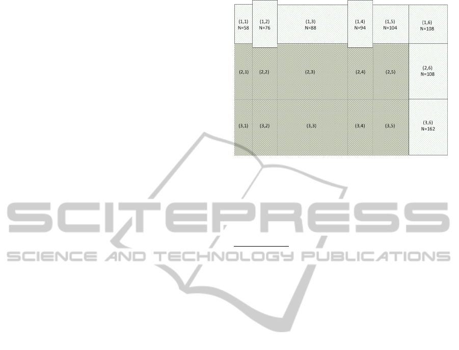
vidually. With the assumption that moving is a lit-
Figure 1: Real map coordinates and grid north direction val-
ues.
tle imprecise, the robot loses information regarding
position after movement and gains information af-
ter sense. In refreshing of the location after sense,
the histogram filtering use Bayes Rule, P(x
i
|Sense) =
P(Sense|x
i
)∗P(x
i
)
P(Sense)
, where P(Sense|x
i
) is the probability of
sense (precision of sense), P(x
i
) is the probability of
location before update, P(Sense) is the sum of proba-
bilities from all fields of the map, the value by which
we normalize all values of the map. The next step of
filtration consists of an update after movement (con-
volution of probability) - it depends on precision of
movement. In the real world the motion is uncer-
tain. Update after movement consists of computing
total probability, P(x
i
) =
∑
i
P(x
j
)∗P(x
i
|x
j
) This is the
probability of location in the field x
i
after movement
from the fields x
j
with fixed precision of motion.
3 REAL LIFE SOLUTION
For experimental reason we have chosen the corri-
dor of a real building and described it in the follow-
ing way. The corridor was split into eight distinctive
available areas - see Fig. 1. Because of magnetic dis-
turbance we consider the map of north direction read-
ings - see Fig. 1. The basic map consists of readings
in four directions (north, south, east and west) from
sonar from central points of all the selected areas, see
Fig. 2 and Tab. 1. Additionally we use the map of
field boundaries which is useful in the convolution of
histogram filtering, which is shown in Fig. 3 and Tab.
2.
3.1 The Disturbance of Sonar Readings
Caused by Magnetic Deviation
In the localization on the real map we encounter the
ICAART2015-InternationalConferenceonAgentsandArtificialIntelligence
342
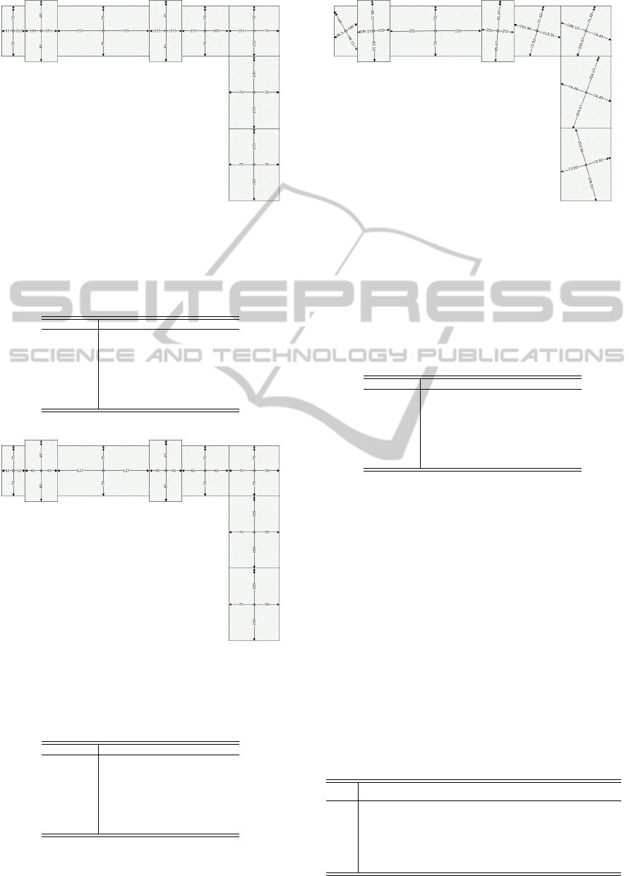
Figure 2: Readings from the sonar on the four map direc-
tions from central points of the map fields - useful for local-
ization; The north direction is marked as a double arrow.
Table 1: Readings from the sonar with a magnetic stable
environment. The north direction is the same for all fields
of the map - see also Fig. 2.
map coord. North South East West
(1, 1) 70 70 255 32
(1, 2) 85 85 255 110
(1, 3) 70 70 255 255
(1, 4) 85 85 255 255
(1, 5) 70 70 205 255
(1, 6) 70 255 70 255
(2, 6) 240 255 70 70
(3, 6) 255 100 70 70
Figure 3: Map boundaries - useful in the convolution of his-
togram filtration; The North direction is marked as double
arrow.
Table 2: Map of field boundaries useful in the convolution
of histogram filtration - see also Fig. 3.
map coord. North South East West
(1, 1) 70 70 32 32
(1, 2) 85 85 45 45
(1, 3) 70 70 127 127
(1, 4) 85 85 45 45
(1, 5) 70 70 65 65
(1, 6) 70 70 70 70
(2, 6) 100 100 70 70
(3, 6) 100 100 70 70
problem of magnetic disturbance mentioned in the In-
troduction. Considering the only one north direction
Figure 4: Readings from the sonar on the four map di-
rections from central points of the map fields with mag-
netic disturbance of north direction; The north direction is
marked as a double arrow; There is assumption that the real
value of north on the map is N = 88 and the robot measure
this value in the (1,3) coordinates.
Table 3: Readings from sonar with magnetic unstable envi-
ronment with the assumption that the real value of north on
the map is N = 88 - see also Fig. 4. The map of magnetic
deviations is shown in Fig 1 and visualization in Fig. 4.
map coord. North South East West
(1, 1) 64 98.15 140.87 36.95
(1, 2) 85.12 85.12 255 109.15
(1, 3) 70 70 255 255
(1, 4) 85.47 85.47 255 255
(1, 5) 72.82 72.82 213.26 253.96
(1, 6) 74.49 204.67 74.49 248.52
(2, 6) 204.67 204.67 74.49 74.49
(3, 6) 72.82 72.82 104.03 253.96
of the map N = 88, from the field (1, 3), in case of
magnetic disturbance shown in Fig. 1 and Fig. 4 we
get the reading on the map shown in Fig 4 and Tab. 3.
As we can see the ability of localization is lowering
and with high deviation the robot can even lose his
position.
In Tab. 4 we have data from sense part of his-
togram filtering, particularly the probability of robot
localization computed with use of similarity measure
from the equation 2. The real measure for all grid
boxes are stored in the Fig. 2 and Tab. 1.
Table 4: Localization ability for all fields after perfect mea-
sure - the north direction is the same for the whole map;
Data from the histogram filter after a single north-south-
east-west(NSEW) sense - in the magnetic stable environ-
ment; for distance measure from equation 2; In the columns
we have ability of location for particular coordinates.
(1, 1) (1, 2) (1, 3) (1, 4) (1, 5) (1, 6) (2, 6) (3, 6)
pos pos pos pos pos pos pos pos
(1, 1) 0.157 0.137 0.137 0.128 0.139 0.124 0.108 0.112
(1, 2) 0.140 0.153 0.138 0.144 0.140 0.131 0.105 0.110
(1, 3) 0.135 0.133 0.159 0.150 0.153 0.111 0.086 0.091
(1, 4) 0.127 0.141 0.152 0.158 0.145 0.118 0.093 0.099
(1, 5) 0.139 0.137 0.155 0.146 0.157 0.115 0.090 0.095
(1, 6) 0.121 0.125 0.110 0.115 0.112 0.161 0.138 0.143
(2, 6) 0.086 0.082 0.069 0.074 0.071 0.113 0.198 0.168
(3, 6) 0.096 0.092 0.079 0.085 0.081 0.126 0.181 0.183
TheLocalizationofMindstormsNXTintheMagneticUnstableEnvironmentBasedonHistogramFiltering
343

We make the assumption that
N
(i, j)
, S
(i, j)
, E
(i, j)
, W
(i, j)
is the basic distance to
obstacles in the field with (i, j) coordinates, and
N
0
, S
0
, E
0
, W
0
is the distance to obstacles after the
single sense of the four directional radar - see Fig.
5. The distance between the original values and the
sensed values has been defined based on two basic
metrics defined as those on equation 1 and 2.
x
(i, j)
= f ield distance
(i, j)
, y = actual sense
d
1
(x
(i, j)
, y) =
A
1
+ B
1
4
(1)
A
1
= (1 −
|N
(i, j)
− N
0
|
N
(i, j)
+ N
0
) + (1 −
|S
(i, j)
− S
0
|
S
(i, j)
+ S
0
)
B
1
= (1 −
|E
(i, j)
− E
0
|
E
(i, j)
+ E
0
) + (1 −
|W
(i, j)
−W
0
|
W
(i, j)
+W
0
)
d
2
(x
(i, j)
, y) =
A
2
+ B
2
2
(2)
A
2
= (1 −
|(N
(i, j)
+ S
(i, j)
) − (N
0
+ S
0
)|
N
(i, j)
+ S
(i, j)
+ N
0
+ S
0
)
B
2
= (1 −
|(E
(i, j)
+W
(i, j)
) − (E
0
+W
0
)|
E
(i, j)
+W
(i, j)
+ E
0
+W
0
)
Figure 5: Demonstration of four directional sonar.
The data from the four directional radar in an un-
stable magnetic environment is shown in Fig. 4 and
Tab 3. The data from histogram filtering in such an
environment is presented in Tab 5.
The result for the metric from equation 1 and mag-
netic stable environment is in Tab. 6, and for magnetic
unstable grid in Tab. 7.
Table 5: Localization ability for all fields with an unstable
magnetic environment; Data from histogram filtering after
a single north-south-east-west sense; for distance measure
from equation 2.
(1, 1) (1, 2) (1, 3) (1, 4) (1, 5) (1, 6) (2, 6) (3, 6)
pos pos pos pos pos pos pos pos
(1, 1) 0.141 0.137 0.137 0.128 0.137 0.129 0.112 0.145
(1, 2) 0.136 0.153 0.138 0.144 0.141 0.136 0.110 0.148
(1, 3) 0.120 0.133 0.159 0.150 0.152 0.115 0.090 0.140
(1, 4) 0.124 0.141 0.152 0.157 0.148 0.123 0.098 0.135
(1, 5) 0.124 0.137 0.155 0.146 0.155 0.119 0.094 0.144
(1, 6) 0.114 0.125 0.110 0.116 0.113 0.154 0.142 0.122
(2, 6) 0.115 0.082 0.069 0.074 0.072 0.106 0.176 0.079
(3, 6) 0.126 0.092 0.079 0.085 0.082 0.119 0.178 0.089
Table 6: Localization ability for all fields with an unstable
magnetic environment; Data from a histogram filter after
a single north-south-east-west(NSEW) sense; for distance
measure from equation 1.
(1, 1) (1, 2) (1, 3) (1, 4) (1, 5) (1, 6) (2, 6) (3, 6)
pos pos pos pos pos pos pos pos
(1, 1) 0.174 0.131 0.129 0.121 0.125 0.093 0.097 0.108
(1, 2) 0.142 0.161 0.136 0.143 0.132 0.108 0.111 0.122
(1, 3) 0.140 0.137 0.160 0.151 0.156 0.127 0.087 0.098
(1, 4) 0.132 0.145 0.152 0.159 0.148 0.126 0.094 0.106
(1, 5) 0.136 0.133 0.155 0.147 0.160 0.131 0.091 0.102
(1, 6) 0.091 0.098 0.114 0.113 0.118 0.178 0.144 0.113
(2, 6) 0.085 0.090 0.070 0.075 0.073 0.128 0.200 0.164
(3, 6) 0.101 0.106 0.084 0.091 0.088 0.108 0.176 0.186
3.2 Lowering Ability of Localization
Caused by Magnetic Deviations
In this subsection we show the effect of magnetic dis-
turbance on localization ability. In the second and
third column of Tab. 8 we have the level of localiza-
tion before and after magnetic disturbance using the
metric from Eq. 2, the data without disturbance is in
Tab. 4 and with magnetic disturbance in Tab. 5. A
similar result for metric from Eq. 1 is shown in the
fourth and fifth column of Tab. 8, data non disturbed
are from Tab. 6, and with magnetic disturbance in Tab
7.
As we can see the localization ability is lower be-
cause of magnetic disturbance and even in this simple
example the robot could lose its position.
In the next subsections we have shown, our exem-
plary, the north direction estimation methods based on
the granules of knowledge in terms of Rough Set The-
ory (Pawlak, 1992), particularly based on the granules
in sense of (Polkowski, 2005) and (Polkowski, 2007)
and simple similarity measures.
3.3 An Estimation of North Direction
after Sense for 4-sonar Radar
Grid = {ob j
(1,1)
, ob j
(1,2)
, ob j
(1,3)
, ob j
(1,4)
, ob j
(1,5)
,
ob j
(1,6)
, ob j
(2,6)
, ob j
(3,6)
}
A = {N, S, E,W, North direction}
ICAART2015-InternationalConferenceonAgentsandArtificialIntelligence
344

Table 7: Localization ability for all fields with an unstable
magnetic environment; Data from a histogram filter after
a single north-south-east-west(NSEW) sense; for distance
measure from equation 1.
(1, 1) (1, 2) (1, 3) (1, 4) (1, 5) (1, 6) (2, 6) (3, 6)
pos pos pos pos pos pos pos pos
(1, 1) 0.154 0.131 0.129 0.120 0.124 0.095 0.101 0.114
(1, 2) 0.135 0.161 0.136 0.143 0.135 0.114 0.118 0.125
(1, 3) 0.123 0.137 0.160 0.151 0.155 0.128 0.094 0.146
(1, 4) 0.123 0.145 0.152 0.159 0.150 0.130 0.101 0.141
(1, 5) 0.128 0.133 0.155 0.147 0.158 0.132 0.097 0.150
(1, 6) 0.109 0.098 0.114 0.113 0.117 0.168 0.137 0.133
(2, 6) 0.105 0.090 0.070 0.075 0.073 0.122 0.182 0.088
(3, 6) 0.123 0.106 0.084 0.091 0.089 0.111 0.169 0.104
Table 8: The effect of magnetic disturbance of localization
ability. In the table we have the difference between the best
locating probability and the second one in decreasing order.
non disturbed disturbed non disturbed disturbed
eq2 eq2 eq1 eq1
(1, 1) 0.017 0.005 0.032 0.019
(1, 2) 0.012 0.012 0.016 0.016
(1, 3) 0.004 0.004 0.005 0.005
(1, 4) 0.008 0.007 0.008 0.008
(1, 5) 0.004 0.003 0.004 0.003
(1, 6) 0.03 0.018 0.047 0.036
(2, 6) 0.017 −0.002(lost) 0.024 0.013
(3, 6) 0.015 −0.059(lost) 0.022 −0.046(lost)
3.3.1 Actual North Direction Estimation Based
on ε - Granules of Knowledge
Our general variant of north direction estimation is
the following,
g
ε
r
gran
(o
sense
) = C
1
C
1
= {ob j
(i, j)
∈ Grid :
IND
ε
(o
sense
, ob j
(i, j)
)
|A| − 1
≥ r
gran
}
where,
ε = min(ε
0
∈ {0.01, 0.02, ..., 1.0} : card(g
ε
0
r
gran
(o
sense
)) ≥ 1)
IND
ε
(o
sense
, ob j
(i, j)
) = C
2
C
2
= {a ∈ {N, S, E,W } :
|a(o
sense
) − a(ob j
(i, j)
)|
a(o
sense
) + a(ob j
(i, j)
)
≤ ε}
in our case r
gran
= 1.0
North a fter sense = C
3
C
3
= {
∑
(North direction(ob j
(i, j)
))
card(g
ε
r
gran
(o
sense
))
: ob j
(i, j)
∈ g
ε
r
gran
(o
sense
)}
Table 9: Original Senses from the central points of Grid
fields with measured north directions; (G, A).
ob j.no. N S E W North direction
ob j
(1,1)
70 70 255 32 58
ob j
(1,2)
85 85 255 110 76
ob j
(1,3)
70 70 255 255 88
ob j
(1,4)
85 85 255 255 94
ob j
(1,5)
70 70 205 255 104
ob j
(1,6)
70 255 70 255 108
ob j
(2,6)
240 255 70 70 108
ob j
(3,6)
255 100 70 70 162
Table 10: Exemplary sense.
N S E W North direction
o
sense
N
sense
S
sense
E
sense
W
sense
N
estimation
3.3.2 Actual North Direction Estimation Based
on Similarity Measures
The equivalent method for similarity measures is the
following,
g
ε
(o
sense
) = {ob j
(i, j)
∈ Grid : d(o
sense
, ob j
(i, j)
) ≤ ε}
ε = max(ε
0
∈ {0.01, 0.02, ..., 1.0} : card(g
ε
0
(o
sense
)) ≥ 1)
North a f ter sense = C
4
C
4
= {
∑
(North direction(ob j
(i, j)
))
card(g
ε
(o
sense
))
: ob j
(i, j)
∈ g
ε
(o
sense
)}
where d is the fixed similarity measure, for example
those from equations 1 and 2.
3.4 Emergency North - Useful in Case
of Mis-localization
The defined emergency north direction consists of
card{Grid} − 2 elements, because the highest and
smallest values are removed from consideration - see
the Eq. 3. The emergency north direction is useful in
case of permanent lose of the position on the map.
Emergency North = C
8
(3)
C
8
=
∑
ob j
(i, j)
∈Grid
0
North
direction(ob j
(i, j)
)
card{Grid} − 2
where,
Grid
0
= {ob j
(i, j)
: ob j
(i, j)
∈ Grid\{ob j
0
(i, j)
: ob j
0
(i, j)
∈
∈ {ob j
00
(i, j)
: max(North direction(ob j
00
(i, j)
)), min(North direction(ob j
00
(i, j)
))}}}
3.5 Cost and Policy to Get Goal
In this subsection we have the computed cost of
movement with assumption that the goal position is
in the coordinates (2, 6) - see Fig. 6, and the policy
of movement (Roy and Thrun, 2002) see Fig. 7. We
made assumption that the cost of a single move is an
equal one, and that the robot can move in the direc-
tion of south, west, north and east. The minimal cost
of reaching the goal is propagated back from the goal
TheLocalizationofMindstormsNXTintheMagneticUnstableEnvironmentBasedonHistogramFiltering
345
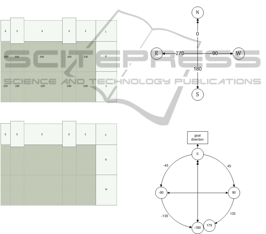
to all fields on the map. Based on the minimal cost of
reaching the goal, we can generate a universal mov-
ing policy, where in the case of more than one pos-
sibility of move, we choose the last conflicted value
with the use of a fixed searching order, south, west,
north and east. We have shown a really simple ex-
ample, with the assumption that the robot can move
precisely in one of four directions. Considering more
complex solution, the agent can move in any direction
with uncertainty, which requires multiple approxima-
tions of this policy ending in the stable point - without
changes in policy.
Figure 6: Cost of reaching the goal in coordinates (2,6).
Figure 7: Universal Policy of reaching the goal in (2,6) co-
ordinates.
3.6 PD-controller
For demonstration purposes we use a robot equipped
with two servo motors, for wheels control, HiTechnic
compass sensor for control of motion in the intended
direction, and a central unit which allows us to con-
trol the robot remotely. The PD-controller (Bennett,
1993) for the steering of Mindstorm NXT robot con-
sists of control of two wheels with fixed velocity. By
building a PD-controller we convert the readings from
the compass in the way shown in Figs. 9 and 10. After
conversion, readings from the compass towards to in-
tended direction are shown in Fig. 8. During conver-
sion we have two variants; the first one occurs when
the intended direction is k < 180 (see Fig. 9), and
the second one occurs when the intended direction is
k >= 180 - see Fig. 10.
We have implemented the controller in C++ with
the use of NXT++ library, (see (NXT++, 2014)). In
the last step we have tuned the parameters of the con-
troller for optimal control.
Readings from compass in degrees, we make
assumption, that value 0 means north, 180 south, 90
east, 270 west.
Figure 8: Compass directions after conversion.
4 SUMMARY OF EXPERIMENTS
To attain the objective we have used the modular li-
brary NXT++ - on the GPLv2 licence. For labo-
ratory use we have developed additional drivers for
the library and released the new version of this li-
ICAART2015-InternationalConferenceonAgentsandArtificialIntelligence
346
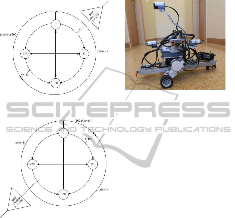
Figure 9: Direction conversion for k < 180, parameter
orient is the original reading from the compass (the value
for conversion).
Figure 10: Direction conversion for k ≥ 180, parameter
orient is the original reading from the compass (the value
for conversion.
brary available in (NXT++, 2014). We have devel-
oped drivers for HiTechnic multiplexers and included
them in the library. As a computing engine we use
a computer connected with the robot via a bluetooth
module. The robot which we have used for experi-
mental purposes is shown in Fig. 11. The software
which we have developed for localization is hosted
on Github - see (RoboGuide.project, 2014). The
exemplary movie from our experiments is available
at (Video.of.histogram.filtering.for.Mindstorms.NXT,
2014). In our experiments we use four-directional
radar from Fig. 5 in move, it is because we want to
see the effect of sense part of histogram filtering. And
the localization ability was better after multiple sense
Figure 11: The construction of our robot - the robot is based
on an aluminium frame (designed by (Artiemjew, 2014)) ;
we have used Lego Mindstorms NXT bricks; there are four
sonar sensors, a magnetic compass and a touch sensor; there
are two HiTechnic sensor multiplexers - the first for digital
and the second for analog sensors; there are two servo mo-
tors in use.
in move than by single four directional sense. As a
metric for sense we use formula from Eq. 2, this met-
ric works best in corridors of building among tested
metrics. The north direction is estimated based on the
method from Sect. 3.3, and the emergency north in
the way from the Sect. 3.4.
5 CONCLUSION
In this work we have designed an algorithm for the
proper localization of a robot in an unstable magnetic
environment. To achieve our goal we have designed a
robot which is based on the Mindstorms NXT parts
with additional multiplexers and a compass sensor
by HiTechnic. We have developed drivers for multi-
plexers in the modular library NXT++ and performed
laboratory and real environment tests. These tests
demonstrate the effectiveness of our approach - the
localization is resistant to magnetic deviations. It
turn out that for such imprecise stuff like Mindstorms
NXT, it is better to use 4 directional radar in move
and metric for localization, which consider overall
distance between walls of the corridor. In our fu-
ture work, we plan to optimize the robo guide library
(RoboGuide.project, 2014) and use it in the net of
corridors. We have also plan to extend our experi-
mental methods to use in the other localization algo-
rithms like particle filtering and Kalman filtering. The
future tasks will be partially supported by Scientific
Robotic Circle of University of Warmia and Mazury -
see (NKR-UWM, 2014).
TheLocalizationofMindstormsNXTintheMagneticUnstableEnvironmentBasedonHistogramFiltering
347

ACKNOWLEDGEMENTS
This research has been supported by a grant 1309-
802 from the Ministry of Science and Higher Educa-
tion of the Republic of Poland, and grant 1309-0883
for young scientists from Department of Mathematics
and Computer Sciences of University of Warmia and
Mazury in Olsztyn.
REFERENCES
Artiemjew, L. (2014). Designer of robot frame - http://
lechart.ovh.org/eng/ and https://www.facebook.com/
lech.artiemjew.
Bennett, S. (1993). A history of control engineering. In
IET, pages 1930–1955.
Dellaert, F., Fox, D., Burgard, W., and Thrun, S. (1999).
Monte carlo localization for mobile robots. In
Robotics and Automation, 1999. Proceedings. 1999
IEEE International Conference on, volume 2, pages
1322–1328 vol.2.
Gozick, B., Subbu, K., Dantu, R., and Maeshiro, T.
(2011). Magnetic maps for indoor navigation. Instru-
mentation and Measurement, IEEE Transactions on,
60(12):3883–3891.
Hart, P., Nilsson, N., and Raphael, B. (1968). A formal basis
for the heuristic determination of minimum cost paths.
Systems Science and Cybernetics, IEEE Transactions
on, 4(2):100–107.
Minorsky, N. (1922). Directional stability of automatically
steered bodies. In J. Amer. Soc. Naval Eng. 34 (2),
pages 280–309.
Navarro, D. and Benet, G. (2009). Magnetic map building
for mobile robot localization purpose. In Proceedings
of the 14th IEEE International Conference on Emerg-
ing Technologies & Factory Automation, ETFA’09,
pages 1742–1745, Piscataway, NJ, USA. IEEE Press.
NKR-UWM (2014). http://www.uwm.edu.pl/nkr/. Robotic
Circle of University of Warmia and Mazury.
NXT++ (2014). NXT++ library 2014 - a library in C++
for programming Mindstorms NXT. By Cory Walker,
extentended by David Butterworth and Piotr Artiem-
jew.
Pawlak, Z. (1992). Rough Sets: Theoretical Aspects of
Reasoning About Data. Kluwer Academic Publishers,
Norwell, MA, USA.
Polkowski, L. (2005). Formal granular calculi based on
rough inclusions. In Granular Computing, 2005 IEEE
International Conference on, volume 1, pages 57–69
Vol. 1.
Polkowski, L. (2007). Granulation of knowledge in decision
systems: The approach based on rough inclusions. the
method and its applications. In Kryszkiewicz, M., Pe-
ters, J., Rybinski, H., and Skowron, A., editors, Rough
Sets and Intelligent Systems Paradigms, volume 4585
of Lecture Notes in Computer Science, pages 69–79.
Springer Berlin Heidelberg.
RoboGuide.project (2014). https://github.com/boxero/
robo-guide.
Roy, N. and Thrun, S. (2002). Motion planning through pol-
icy search. In Intelligent Robots and Systems, 2002.
IEEE/RSJ International Conference on, volume 3,
pages 2419–2424 vol.3.
Suksakulchai, S., Thongchai, S., Wilkes, D., and Kawa-
mura, K. (2000). Mobile robot localization using an
electronic compass for corridor environment. In Sys-
tems, Man, and Cybernetics, 2000 IEEE International
Conference on, volume 5, pages 3354–3359 vol.5.
Video.of.histogram.filtering.for.Mindstorms.NXT
(2014). NXT histogram filtering: http://youtu.be/
Im5IYMRbAp0. by Piotr Artiemjew.
ICAART2015-InternationalConferenceonAgentsandArtificialIntelligence
348
