
Exploration Versus Exploitation Trade-off in Infinite Horizon Pareto
Multi-armed Bandits Algorithms
Madalina Drugan and Bernard Manderick
Artificial Intelligence Lab, Vrije Universiteit Brussel, Pleinlaan 2, 1050 Brussels, Belgium
Keywords:
Multi-armed Bandits, Multi-objective Optimisation, Pareto Dominance Relation, Infinite Horizon Policies.
Abstract:
Multi-objective multi-armed bandits (MOMAB) are multi-armed bandits (MAB) extended to reward vectors.
We use the Pareto dominance relation to assess the quality of reward vectors, as opposite to scalarization
functions. In this paper, we study the exploration vs exploitation trade-off in infinite horizon MOMABs
algorithms. Single objective MABs explore the suboptimal arms and exploit a single optimal arm. MOMABs
explore the suboptimal arms, but they also need to exploit fairly all optimal arms. We study the exploration vs
exploitation trade-off of the Pareto UCB1 algorithm. We extend UCB2 that is another popular infinite horizon
MAB algorithm to rewards vectors using the Pareto dominance relation. We analyse the properties of the
proposed MOMAB algorithms in terms of upper regret bounds. We experimentally compare the exploration
vs exploitation trade-off of the proposed MOMAB algorithms on a bi-objective Bernoulli environment coming
from control theory.
1 INTRODUCTION
Multi-armed bandits (MAB) is a machine learning
paradigm used to study and analyse resource alloca-
tion in stochastic and noisy environments. The multi-
armed bandit problem considers multi-objective re-
wards and imports techniques from multi-objective
optimisation into the multi-armed bandits algorithms.
We call this the multi-objective multi-armed bandits
(MOMAB) problem and it is an extension of the stan-
dard MAB-problem to reward vectors.
1
MOMAB
also has K arms, K ≥ 2, and let I the set of these K
arms. But since we have multiple objectives, a ran-
dom vector of rewards is received, one component per
objective, whenone of the arms is pulled. The random
vectors have a stationary distribution with support in
the D-dimensional hypercube [0,1]
D
but the vector of
true expected rewards µ
i
= (µ
1
i
,...,µ
D
i
), where D is
the number of objectives, is unknown. All rewards X
i
t
obtained from any arm i are independently and identi-
cally distributed according to an an unknownlaw with
unknown expectation vector µ
i
= (µ
1
i
,...,µ
D
i
). Re-
ward values obtained from different arms are also as-
1
Some of these techniques were also imported in other
related learning paradigms: multi-objective Markov Deci-
sion Processes Lizotte et al. (2010); Wiering and de Jong
(2007), and multi-objective reinforcement learning van
Moffaert et al. (2013); Wang and Sebag (2012).
sumed to be independent. A MAB algorithm chooses
the next machine to play based on the sequence of
past plays and obtained reward values.
MOMAB leads to important differences com-
pared to the standard MAB. Pareto dominance Zitzler
et al. (2003) allows to maximize the reward vectors
directly in the vector reward space. A reward vector
can optimize one objective and be sub-optimal in the
other objectives, leading to many vector rewards of
the same quality. Thus, there could be several arms
considered to be the best according to their reward
vectors. We call the set of optimal arms of the same
quality the Pareto front. An adequate regret definition
for the Pareto MAB algorithm measures the distance
between a suboptimal reward vector and the Pareto
front. We call this class of algorithms the Pareto MAB
problem.
The main goal of this paper is to study the explo-
ration vs exploitation trade-off in several Pareto MAB
algorithms. Exploration means pulling the subopti-
mal arms that might have been unlucky, whereas ex-
ploitation means pulling as much as possible the op-
timal arms. The exploration vs exploitation trade-
off is different for single objective MABs and for
MOMABs. For single objective MABs, we are con-
cerned with the exploration of the suboptimal arms
and the exploitation of a single optimal arm. In
MOMABs, by design, we should pull equally often
66
Drugan M. and Manderick B..
Exploration Versus Exploitation Trade-off in Infinite Horizon Pareto Multi-armed Bandits Algorithms.
DOI: 10.5220/0005195500660077
In Proceedings of the International Conference on Agents and Artificial Intelligence (ICAART-2015), pages 66-77
ISBN: 978-989-758-074-1
Copyright
c
2015 SCITEPRESS (Science and Technology Publications, Lda.)

all the arms in the Pareto front. Thus, the exploitation
now means the fair usage of Pareto optimal arms.
This difference in exploitation vs exploration
trade-off reflects on all aspects of Pareto MAB algo-
rithmic design. There are two regret metrics for the
MOMAB algorithms Drugan and Nowe (2013). One
performance metric, i.e. the Pareto projection regret
metric, measures the amount of times any Pareto opti-
mal arm is used. Another performance metric, i.e. the
Pareto variance regret metric, measures the variance
in using all Pareto optimal arms. Background infor-
mation on MOMABs, in general, and Pareto MABs,
in particular, are given in Section 2.
We propose several Pareto MAB algorithms that
are an extension of the classical single objectiveMAB
algorithms, i.e. UCB1 and UCB2 Auer et al. (2002),
to reward vectors. The proposed algorithms focus
on either the exploitation or the exploration mecha-
nisms. We consider the Pareto UCB1 Drugan and
Nowe (2013) to be an exploratory variant of this al-
gorithm because each round only one Pareto optimal
arm is pulled. In Section 3, we propose an exploita-
tive variant of the Pareto UCB1 algorithm where, each
round, all the Pareto optimal arms are pulled. We
show that the analytical properties, i.e. upper confi-
dence bound of the Pareto projection regret, for the
exploitative Pareto UCB1 are improved when com-
pared with the exploratory variant of the same algo-
rithm because this bound is independent of the cardi-
nality of the Pareto front.
Section 4 proposes two multi-objective variants of
UCB2 correspondingto the two exploitation vs explo-
ration mechanisms described before. The exploita-
tive Pareto UCB2 is an extension of UCB2 where,
each epoch, all the Pareto optimal arms are pulled
equally often. This algorithm is introduced in Sec-
tion 4.1. The exploratory Pareto UCB2 algorithm, see
Section 4.2, pulls each epoch a single Pareto optimal
arm. We compute the upper bound of the Pareto pro-
jection regret for the exploitative Pareto UCB2 algo-
rithm.
Our motivating example is a bi-objective wet
clutch Vaerenbergh et al. (2012) that is a system with
one input characterised by a hard non-linearity when
the piston of the clutch gets in contact with the fric-
tion plates. These clutches are typically used in power
transmissions of off-road vehicles, which operate un-
der strongly varying environmental conditions. The
validation experiments are carried out on a dedicated
test bench, where an electro-motor drives a flywheel
via a torque converser and two mechanical transmis-
sions. The goal is to learn by minimising simulta-
neously: i) the optimal current profile to the electro-
hydraulic valve, which controls the pressure of the
oil to the clutch, and ii) the engagement time. The
output data is stochastic because the behavior of the
machine varies with the surrounding temperature that
cannot be exactly controlled. Section 5 experimen-
tally compares the proposed MOMAB algorithms on
a bi-objective Bernoulli reward distribution generated
on the output solutions of the wet clutch.
Section 6 concludes the paper.
2 THE MULTI-OBJECTIVE
MULTI-ARMED BANDITS
PROBLEM
We consider the general case where a reward vector
can be better than another reward vector in one objec-
tive, and worse in another objective. Expected reward
vectors are compared according to the Pareto domi-
nance relation Zitzler et al. (2003).
The following dominance relations between two
vectors µ and ν are used. A vector µ is dominating,
another vector ν, ν ≺ µ, if and only if there exists at
least one objective o for which ν
o
< µ
o
and for all
other objectives j, j 6= i, we have ν
j
≤ µ
j
. A reward
vector µ is incomparable with another vector ν, νkµ,
if and only if there exists at least one objective o for
which ν
o
< µ
o
, and there exists another objective j,
j 6= i, for which ν
j
> µ
j
. Finally, the vector µ is non-
dominated by ν, ν 6≻ µ, if and only if there exists at
least one objective o for which ν
o
< µ
o
. Let A
∗
be the
Pareto front, i.e. non-dominated by any arm in A.
2.1 The Exploration vs Exploitation
Trade-off in Pareto MABs
A Pareto MAB-algorithm selects an arm to play based
on the previous plays and the obtained reward vec-
tors and it tries to maximize the total expected reward
vectors. The goal of a MOMAB algorithm is to si-
multaneously minimise the regret of not selecting the
Pareto optimal arms by fairly playing all the arms in
the Pareto front.
In order to measure the performance of these al-
gorithms, we define two Pareto regret metrics. The
first regret metric measures the loss in pulling arms
that are not Pareto optimal and is called the Pareto
projection regret. The second metric, the Pareto vari-
ance regret, measures the variance
2
in pulling each
arm from the Pareto front A
∗
.
2
Not to be confused with the variance of random vari-
ables.
ExplorationVersusExploitationTrade-offinInfiniteHorizonParetoMulti-armedBanditsAlgorithms
67

The Pareto projection regret expresses the ex-
pected loss due to the play of suboptimal arms. For
this purpose, it uses the Euclidean distance between
the mean reward vector µ
i
of an arm i and its projec-
tion ν
i
into the Pareto front. This projection is ob-
tained as follows: A vector ε
i
with equal components
ε
i
, i.e. ε
i
= (ε
i
,ε
i
,··· ,ε
i
), is added to µ
i
such that ε
i
is the smallest value for which ν
i
= µ
i
+ ε
i
becomes
Pareto optimal. The Euclidean distance ∆
i
between µ
i
and its projection ν
i
into the Pareto front equals:
∆
i
= kν
i
−µ
i
k
2
= kε
i
k
2
=
√
Dε
i
(1)
where the last equality holds because we have D ob-
jectives and all components of ε
i
are the same.
Since by definition ∆
i
is always non-negative, the
resulting regret is also non-negative. Note that the for
a Pareto optimal arm ν
i
= µ
i
and ∆
i
= 0.
Let T
i
(n) be the number of times that arm i has
been played after n plays in total. Then the Pareto
projection regret R
p
(n) after n plays is defined as:
R
p
(n) =
∑
i6∈A
∗
∆
i
E[T
i
(n)] (2)
where ∆
i
is defined in Equation 1 and where E is the
expectation operator. A similar regret metric was in-
troduced in Drugan and Nowe (2013).
The Pareto variance regret metric measures the
variance of a Pareto-MAB algorithm in pulling all op-
timal arms. Let T
∗
i
(n) be the number of times an op-
timal arm i is pulled during n total arm pulls. Let
E[T
∗
i
(n)] the expected number of times the Pareto op-
timal arm i is pulled. The Pareto variance regret is
defined as
R
v
(n) =
1
|A
∗
|
∑
i∈A
∗
(E[T
∗
i
(n)] −E[T
∗
(n)]/|A
∗
|)
2
(3)
where E[T
∗
(n)] is the expected number of times that
any Pareto optimal arm is selected, and |A
∗
| is the
cardinality of the Pareto front A.
If all Pareto optimal arms are played in a fair way,
i.e. an equal number of times, then R
v
(n) is mini-
mized. For a perfect fair, or equal, usage of the Pareto
optimal arms, we have R
v
(n) ← 0. If a Pareto MAB-
algorithm identifies only a subset of A
∗
, then R
v
(n) is
large. A similar measure, called unfairness, was pro-
posed in Drugan and Nowe (2013) to measure vari-
ance of a Pareto-MAB algorithm in pulling all Pareto
optimal arms.
Algorithm 1: Exploitative Pareto UCB1.
1: Play each arm i once
2: t ← 0; n ← K; n
i
← 1, ∀i
3: while the stopping criteria is NOT met do
4: t ←t + 1
5: Select the Pareto front at the round t, A
∗(t)
,
such that ∀i ∈ A
∗(t)
the index ˆµ
i
+
r
2ln(n
4
√
D)
n
i
is non-dominated
6: Pull each arm i once, where i ∈A
∗(t)
7: ∀i ∈ A
∗(t)
, update ˆµ
i
, and n
i
← n
i
+ 1
8: n ← n+ |A
∗(t)
|
9: end while
3 EXPLORATION VS
EXPLOITATION TRADE-OFF
IN PARETO UCB1
The Pareto UCB1 algorithm Drugan and Nowe(2013)
is an UCB1 algorithm using the Pareto dominance
relation to partially order the reward vectors. Like
for the classical single-objective UCB1 Auer et al.
(2002), the index for a Pareto UCB1 algorithm has
two terms: the mean reward vector, and the sec-
ond term related to the size of a one-sided confi-
dence interval of the average reward according to the
Chernoff-Hoeffding bounds.
In this section, we propose a Pareto UCB1 algo-
rithm with an improved exploration vs exploitation
trade-off because its performance does not depend on
the size of Pareto front. In each round, all the Pareto
optimal arms are pulled once instead of pulling only
one arm. This means that the proposed Pareto UCB1
algorithm has an aggressive exploitation mechanism
of Pareto optimal arms that improves it upper regret
bound. We denote this algorithm with the exploitative
Pareto UCB1 algorithm as opposite with the Pareto
UCB1 algorithm from Drugan and Nowe (2013), de-
noted as exploratory Pareto UCB1 algorithm.
3.1 Exploitative Pareto UCB1
The pseudo-code for the exploitative Pareto UCB1 is
given in Algorithm 1. To initialise the algorithm, each
arm is played once. Let ˆµ
i
be the estimation of the true
but unknown expected reward vector µ
i
of an arm i.
In each iteration, we compute for each arm i its index,
i.e. the sum of the estimated reward vector ˆµ
i
and the
associated confidence value of arm i
ICAART2015-InternationalConferenceonAgentsandArtificialIntelligence
68

ˆµ
i
+
s
2ln(n
4
√
D)
n
i
=
ˆµ
1
i
+
s
2ln(n
4
√
D)
n
i
,... , ˆµ
D
i
+
s
2ln(n
4
√
D)
n
i
At each time step t, the Pareto front A
∗(t)
is deter-
mined using the indexes ˆµ
i
+
r
2ln(n
4
√
D)
n
i
. Thus, for
all arms not in the Pareto front i 6∈ A
∗(t)
, there exists a
Pareto optimal arm h ∈ A
∗(t)
that dominates arm i:
ˆµ
h
+
s
2ln(n
4
√
D)
n
h
≻ ˆµ
i
+
s
2ln(n
4
√
D)
n
i
Each iteration, the exploitative Pareto UCB1 al-
gorithm selects all Pareto optimal arm from A
∗(t)
and
pull them. Thus, by design, this algorithm is fair in
selecting Pareto optimal arms. Next, the estimated
vector of the selected arm ˆµ
h
and the corresponding
counters are updated. A possible stopping criteria is a
given fix number of iterations.
The following theorem provides an upper bound
for the Pareto regret of the efficient Pareto UCB1
strategy. The only difference is that a suboptimal arm
is pulled |A
∗
| times less often than in the exploratory
Pareto UCB1 algorithm. This fact is reflected by the
multiplicative constant,
4
√
D, in the index of the algo-
rithm.
Theorem 1. Let exploitative Pareto UCB1 from Al-
gorithm 1 be run on a K-armed D-objective bandit
problem, K > 1, having arbitrary reward distributions
P
1
,... P
K
with support in [0,1]
D
. Consider the Pareto
regret defined in Equation 1. The expected Pareto pro-
jection regret of after any number of n plays is at most
∑
i6∈A
∗
8·ln(n
4
√
D)
∆
i
+ (1+
π
2
3
) ·
∑
i6∈A
∗
∆
i
Proof. The prove follows closely the prove from Dru-
gan and Nowe (2013). Let X
i,1
,...,X
i,n
be random D-
dimensional variables generated for arm i with com-
mon range [0,1]
D
. The expected reward vector for the
arm i after n pulls is
¯
X
i,n
= 1/n ·
n
∑
t=1
X
i,t
⇒ ∀j,
¯
X
j
i,n
= 1/n ·
n
∑
t=1
X
j
i,t
Chernoff-Hoeffding bound. We use a straight-
forward generalization of the standard Chernoff-
Hoeffding bound for D dimensional spaces. Con-
sider that ∀j, 1 ≤ j ≤D, IE[X
j
i,t
|X
j
i,1
,... ,X
j
i,t−1
] = µ
j
i
.
There,
¯
X
i,n
6≺µ
i
+a if there exists at least a dimension
j for which
¯
X
j
i,n
> µ
j
i
+ a. Translated in Chernoff-
Hoeffding bound, using union bound, for all a ≥ 0,
we have
IP{
¯
X
i,n
6≺ µ
i
+ a
} = (4)
IP{
¯
X
1
i,n
> µ
1
i
+ a
∨... ∨
¯
X
D
i,n
> µ
D
i
+ a
}≤ De
−2na
2
Following the same line of reasoning
IP{
¯
X
1
i,n
< µ
1
i
−a
∨... ∨
¯
X
D
i,n
< µ
D
i
−a
}≤ De
−2na
2
(5)
Let ℓ > 0 an arbitrary number. We take c
t,s
=
q
2·ln(t
4
√
D)/s, and we upper bound T
i
(n) on any
sequence of plays by bounding for each t ≥ 1 the in-
dicator (I
t
= i). We have (I
t
= i) = 1 if arm i is played
at time t and (I
t
= i) = 0 otherwise. We use the super-
script ∗ when we mean a Pareto optimal arm. Thus,
T
∗
h
(n) means that the arm h is Pareto optimal, h ∈A
∗
.
Then,
T
i
(n) = 1+
n
∑
t=K+1
{I
t
= i} ≤
ℓ +
n
∑
t=K+1
{I
t
= i,T
i
(t −1) ≥ ℓ}≤ ℓ +
n
∑
t=K+1
1
|A
∗
|
·
|A
∗
|
∑
h=1
{
¯
X
∗
h,T
∗
h
(t−1)
+c
t−1,T
∗
h
(t−1)
6≻
¯
X
i,T
i
(t−1)
+c
t−1,T
i
(t−1)
}
≤
s
∗
h
← T
∗
h
(t −1)
s
i
← T
i
(t −1)
ℓ+
∞
∑
t=1
t−1
∑
s=1
t−1
∑
s
i
=ℓ
1
|A
∗
|
|A
∗
|
∑
h=1
{
¯
X
∗
h,s
∗
h
+ c
t−1,s
∗
h
6≻
¯
X
i,s
i
+ c
t−1,s
i
}
(6)
From the straightforward generalization of
Chernoff-Hoeffding bound to D objectives, we have
that
IP{
¯
X
(t)
i
6≺ µ
i
+ c
(t)
s
} ≤
D
D
·t
−4
= t
−4
and
IP{
¯
X
∗(t)
h
6≻ µ
∗
h
−c
(t)
s
∗
h
} ≤t
−4
For s
i
≥
8·ln(n
4
√
D)
∆
2
i
, we have that
ν
∗
i
−µ
i
−2·c
t,s
i
= ν
∗
i
−µ
i
−2·
s
2·ln(n
4
√
D)
s
i
≥ ν
∗
i
−µ
i
−∆
i
Thus, we take ℓ = ⌈
8·ln(n
4
√
D)
∆
2
i
⌉, and we have
IE[T
i
(n)] ≤ ⌈
8·ln(n
4
√
D)
∆
2
i
⌉+
∞
∑
t=1
t−1
∑
s=1
∑
s
i
=⌈
8·ln(n
4
√
D)
∆
2
i
⌉
|A
∗
|
∑
h=1
(IP{
¯
X
∗(t)
h
6≻ µ
∗
h
−c
(t)
s
∗
h
}+ IP{
¯
X
(t)
i
6≺ µ
i
+ c
(t)
s
i
})
ExplorationVersusExploitationTrade-offinInfiniteHorizonParetoMulti-armedBanditsAlgorithms
69

≤
8·ln(n·
4
√
D)
∆
2
i
+ 1+
∞
∑
t=1
t
∑
s=1
t
∑
s
i
=1
|A
∗
|
∑
h=1
t
−4
t
−4
|A
∗
|
=
≤
8·ln(n
4
√
D)
∆
2
i
+ 1+ 2 ·
∞
∑
t=1
t
2
·|A
∗
|
t
−4
|A
∗
|
=
8·ln(n
4
√
D)
∆
2
i
+ 1+ 2 ·
∞
∑
t=1
t
−2
Approximating the last term with the Riemann
zeta function ζ(2) =
∑
∞
t=1
t
−2
≈
π
2
6
we obtain the
bound from the theorem.
For a suboptimal arm i, we have IE[T
i
(n)] ≤
8
∆
2
i
ln(n
4
√
D) plus a small constant. Like for the stan-
dard UCB1, the leading constant is 8/∆
2
i
and the ex-
pected upper bound of the Pareto regret for the ex-
ploitative Pareto UCB1 is logarithmic in the number
of plays n. Unlike exploratory Pareto UCB1 Drugan
and Nowe (2013), this expected bound does not de-
pend on the cardinality of the Pareto front A
∗
. This is
an important improvement for the exploratory Pareto
UCB1 since the size of the Pareto optimal arms is: i)
usually not known beforehand, and ii) increases with
the number of objectives.
Note that the algorithm reduces to the standard
UCB1 for D = 1. Thus, exploitative Pareto UCB1
performs similarly with the standard UCB1 for small
number of objectives. Consider that almost all the
arms K are Pareto optimal arms, |A |
∗
≈ K. Then,
each iteration, the exploitative Pareto UCB1 algo-
rithm pulls once (almost) all arms.
3.2 Exploratory Pareto UCB1
The exploratory version of Pareto UCB1 algorithm
was introduced in Drugan and Nowe (2013) and it
is a straightforward extension of the UCB1 algorithm
to reward vectors. The main difference between the
exploratory Pareto UCB1 and the exploitative Pareto
UCB1, cf Algorithm 1, is in lines 6 −8 of the algo-
rithm. For the exploratory Pareto UCB1 algorithm,
each iteration, a single Pareto optimal arm is selected
uniformly at random and pulled. The counters are up-
dated accordingly, meaning that n ←n + 1.
Another difference is the index associated to the
mean vector that is larger than for the exploitative
Pareto UCB1. Thus, the Pareto set is now the non-
dominated vectors ˆµ
i
+
r
2ln(n
4
√
D|A
∗
|)
n
i
.
The regret bound for the exploratoryPareto UCB1
algorithm using Pareto regrets is logarithmic in the
number of plays for a suboptimal arm and in the size
of the reward vectors, D. In addition, this confidence
bound is also logarithmic in the cardinality of Pareto
Algorithm 2: Exploitative Pareto UCB2.
Require: 0 < α < 1; the length of a epoch r is an
exponential function τ(r) = ⌈(1+ α)
r
⌉
1: Play each arm once
2: n ←K; r
i
← 1, ∀i
3: while the stopping condition is NOT met do
4: Select the Pareto front at the epoch r, A
∗(r)
,
such that ∀i ∈A
∗(r)
, the index ˆµ
i
+a
τ(r
i
)
n
is non-
dominated
5: for all i ∈A
∗(t)
do
6: Pull the arm i exactly τ(r
i
+ 1) −τ(r
i
)
7: Update ˆµ
i
, and r
i
← r
i
+ 1
8: r ← r+ 1 and n ← n+ τ(r+ 1) −τ(r)
9: end for
10: end while
front, |A
∗
|. This indicates a poor behavior of the ex-
ploratory Pareto UCB1 for a large Pareto front ap-
proaching the number of total arms, which is usually
the case for large number of objectives.
4 THE EXPLORATION VS
EXPLORATION TRADE-OFF IN
PARETO UCB2
In this section, we propose Pareto MAB algorithms
that extend of the standard UCB2 algorithm to reward
vectors. Like for the standard UCB2, these Pareto
UCB2 algorithms play the optimal arms in epochs.
These epochs are exponential with the number of
plays in order to allow the gradual selection of good
arms to be played longer each epoch. In single objec-
tive MABs, the UCB2 algorithm is acknowledged to
have a better upper regret bound than the UCB1 algo-
rithm Auer et al. (2002). We show that Pareto UCB2
algorithms have a better upper Pareto projection re-
gret bound than the Pareto UCB1 algorithms, consid-
ering the same exploitation vs exploration trade-off.
The first proposed Pareto UCB2 algorithm, see
Section 4.1, plays in an epoch all Pareto optimal arms
equally often. We call this algorithm an exploitative
Pareto UCB2 algorithm. The second Pareto UCB2
algorithm introduced in Section 4.2 plays only one
Pareto optimal arm per epoch. We call this algorithm
an exploratory Pareto UCB2 algorithm.
4.1 Exploitative Pareto UCB2
In this section, we present the exploitative Pareto
UCB2 algorithm and we analyze its upper confidence
bound. The pseudo-code for this algorithm is given in
Algorithm 2.
ICAART2015-InternationalConferenceonAgentsandArtificialIntelligence
70

As an initial step, we play each arm once. The
plays are divided in epochs, r, of exponential length
until a stopping criteria is met a fix number of arm’
pulls. The length of an epoch is an exponential func-
tion τ(r) = ⌈(1+α)
r
⌉. In each epoch, we compute for
each arm i an index given by with the sum of expected
rewards plus a second term for the confidence value
ˆµ
i
+ a
τ(r
i
)
n
←
ˆµ
1
i
+ a
τ(r
i
)
n
,... , ˆµ
D
i
+ a
τ(r
i
)
n
where a
τ(r
i
)
n
=
q
(1+α)·ln(e·n/(D·τ(r
i
)))
2·τ(r
i
)
, and r
i
is the
number of epochs played by the arm i. A Pareto front
A
∗(r)
is selected from all vectors ˆµ
i
+ a
τ(r
i
)
n
. Thus,
∀i ∈A , exists h ∈A
∗(t)
, such that we have
ˆµ
h
+ a
τ(r
h
)
n
≻ ˆµ
i
+ a
τ(r
i
)
n
Each arm i ∈ A
∗(t)
is selected and played τ(r
i
+ 1) −
τ(r
i
) consecutive times. The mean value and the
epoch counter for all Pareto optimal arms are updated
accordingly, meaning that r
i
←r
i
+1. The total epoch
counter, r, and the total number of arms’ pulls n are
also updated.
The following theorem bounds the expected regret
for the Pareto UCB2 strategy from Algorithm 2.
Theorem 2. Let exploitative Pareto UCB2 from Al-
gorithm 2 be run on K-armed bandit, K > 1, having
arbitrary reward distributions P
1
,... P
K
with support
in [0,1]
D
. Consider the regret defined in Equation 1.
The expected regret of a strategy π after any num-
ber of n ≥max
ˆµ
i
/∈A
∗
D
2·∆
2
i
plays is at most
∑
i:ˆµ
i
/∈A
∗
D·
(1+ α) ·(1+ 4·α) ·ln(2·e·∆
2
i
·n/D)
2·∆
i
+
c
α
∆
i
where
c
α
= 1+
D
2
·(1+ α) ·e
α
2
+
D
α+2
·
α+ 1
α
(1+α)
·
1+
11·D·(1+ α)
5·α
2
·ln(1+ α)
Proof. This prove is based on the homologue prove
of Auer et al. (2002). We consider n ≥
D
2·∆
2
i
, for all i.
From the definition of τ(r) we can deduce that τ(r) ≤
τ(r−1) ·(1−α) + 1.
Let τ(˜r
i
) be the largest integer such that
τ(˜r
i
−1) ≤
D·(1+ 4·α) ·ln(2·e·n·∆
2
i
/D)
2·∆
2
i
We have that for an suboptimal arm i
T
i
(n) ≤ 1+
1
|A
∗
|
·
∑
r≥1
(τ(r) −τ(r−1))·{arm i finished its r-th epoch }
≤ τ(˜r
i
) +
1
|A
∗
|
·
∑
r>˜r
i
(τ(r) −τ(r−1))·{arm i finished its r-th epoch }
The assumption n ≤ D/(2 ·∆
2
i
) implies ln(2e ·
n∆
2
i
/D) ≥ 1. Therefore, for r > ˜r
i
, we have
τ(r−1) >
D·(1+ 4α) ·ln(2e·n∆
2
i
/D)
2·∆
2
i
(7)
and
a
τ(r−1)
n
=
s
(1+ α)ln(e·n/(D·τ(r−1)))
2τ(r−1)
≤
Eq 7
∆
i
√
D
·
s
(1+ α)ln(e·n/(D·τ(r−1)))
(1+ 4α)ln(2e·n∆
2
i
/D)
≤
∆
i
√
D
·
s
(1+ α)ln(2e·n∆
2
i
/D))
(1+ 4α)ln(2e·n∆
2
i
/D)
≤
∆
i
√
D
·
r
1+ α
1+ 4α
Because a
τ(r)
t
is increasing in t, by definition, if the
suboptimal arm j finishes to play the r-th epoch then
∀h, 1 ≤ h ≤ |A
∗(r)
|, ∃s
h
≥ 0, ∃t ≥ τ(r −1) + τ(s
h
)
such that arm i is non-dominated by any of the Pareto
optimal arms in |A
∗(r)
|. This means that
¯
X
∗τ(s
h
)
h
+ a
s
h
t
6≻
¯
X
τ(r−1)
i
+ a
τ(r−1)
t
implies that one of the following conditions holds
¯
X
τ(r−1)
i
+ a
τ(r−1)
n
6≺ν
∗
i
−
α·∆
i
√
D·2
or
¯
X
∗τ(s
h
)
h
+ a
τ(s
h
)
τ(r−1)+τ(s
h
)
6≻ µ
∗
h
−
α·∆
i
√
D·2
Then,
IE[T
i
(n)] ≤ τ(˜r
i
) +
∑
r≥˜r
i
τ(r) −τ(r−1)
|A
∗
|
· (8)
|A
∗
|
∑
h=1
IP{
¯
X
τ(r−1)
i
+ a
τ(r−1)
n
6≺ν
∗
i
−
α·∆
i
√
D·2
}+
∑
i≥0
∑
r≥1
τ(r) −τ(r−1)
|A
∗
|
·
|A
∗
|
∑
h=1
IP{
¯
X
τ(r−1)
s
h
+ a
τ(s
h
)
τ(r−1)−τ(s
h
)
6≻ µ
∗
h
−
α·∆
i
√
D·2
}
ExplorationVersusExploitationTrade-offinInfiniteHorizonParetoMulti-armedBanditsAlgorithms
71

Let’s expand Inequation 8 using Chernoff and
union bound. For the first term between the paren-
thesis, we have that
IP{
¯
X
τ(r−1)
i
+ a
τ(r−1)
n
6≺ ν
∗
i
−
α·∆
i
√
D·2
} =
D
∑
j=1
IP{
¯
X
jτ(r−1)
i
+ a
τ(r−1)
n
> µ
j
i
+ ∆
i
−
α·∆
i
√
D·2
} ≤
D·e
−2·τ(r−1)·∆
2
i
·(1−
α
2·
√
D
−
1
√
D
·
1+α
1+4·α
)
2
≤
α<1/10
D·e
−
τ(r−1)·∆
2
i
·α
2
2·D
If g(x) =
x−1
1+α
and c =
∆
2
i
·α
2
D
, and g(x) ≤ τ(r−1) then
∑
r≥1
τ(r) −τ(r−1)
|A
∗
|
·
|A
∗
|
∑
h=1
IP{
¯
X
τ(r−1)
i
+ a
τ(r−1)
n
6≺ν
∗
i
−
α·∆
i
√
D·2
} ≤
∑
r≥1
∑
i≥0
τ(r) −τ(r−1)
|A
∗
|
·
|A
∗
|
∑
h=1
D·e
−τ(r−1)·∆
2
i
·α
2
/D
=
D·|A
∗
|·
∑
r≥1
∑
i≥0
τ(r) −τ(r−1)
|A
∗
|
·e
−τ(r−1)·∆
2
i
·α
2
/D
≤
D
|A
∗
|
·|A
∗
|·
Z
∞
0
e
−c·g(x)
dx ≤
D
2
·(1+ α) ·e
∆
2
i
·α
2
Let’s now expand the second term of the parenthe-
sis in Inequation 8
IP{
¯
X
τ(r−1)
s
+ a
τ(s)
τ(r−1)−τ(s)
6≻ µ
∗
h
−
α·∆
i
√
D·2
} =
D
∑
j=1
IP{
¯
X
jτ(r−1)
s
+ a
τ(s)
τ(r−1)−τ(s)
< µ
j∗
h
−
α·∆
i
√
D·2
} ≤
D·e
−τ(i)·
α
2
·∆
2
i
D·2
·e
−(1+α)·ln
e·(τ(r−1)+τ(i))
D·τ(i)
≤
D
α+2
·e
−τ(i)·
α
2
·∆
2
i
D·2
·
τ(r−1) + τ(i)
τ(i)
−(1+α)
Thus,
∑
i≥0
∑
r≥1
τ(r) −τ(r −1)
|A
∗
|
·
|A
∗
|
∑
h=1
IP{
¯
X
τ(r−1)
s
+ a
τ(s)
τ(r−1)−τ(s)
6≻ µ
∗
h
−
α·∆
i
√
D·2
} ≤
D
α+2
·
∑
i≥0
e
−τ(i)·
α
2
·∆
2
i
D·2
·
Z
∞
0
1+
x−1
(1+ α) ·τ(i)
−(1+α)
dx ≤
D
α+2
·
α
(1+ α) −1
·
α+ 1
α
(1+α)
·
∑
i≥0
τ(i) ·e
−τ(i)·
α
2
·∆
2
i
D·2
Following the rationale from the prove of Theo-
rem 2 from Auer et al. (2002), we can bound further
the first term of Inequation 8 to
∑
i≥0
τ(i) ·e
−τ(i)·
α
2
·∆
2
i
D·2
≤ 1+
11·D·(1+ α)
5α
2
·∆
2
i
·ln(1+ α)
Using the bounds above, we now bound the ex-
pected regret for an arm i in Algorithm 2
IE[T
i
(n)] ≤ τ(˜r
i
) −1 +
c
α
∆
2
i
where
c
α
= 1+
D
2
·(1+ α) ·e
α
2
+
D
α+2
·
α+ 1
α
(1+α)
·
1+
11·D·(1+ α)
5·α
2
·ln(1+ α)
and the upper bound on τ( ˜r
i
)
τ( ˜r
i
) ≤ τ(˜r
i
−1)(1+ α) + 1≤
D·(1+ α) ·(1+ 4α) ·ln(2en∆
2
i
/D)
2·∆
2
i
+ 1
This concludes our prove.
The bound of the expected regret for Pareto UCB2
is the similar with the bound for the standard UCB2
within a constant given by the number of objectives
D. The intuition is that now the algorithm has to run D
times longer to achieve a similar regret bound for the
Pareto UCB2. For α small, the Pareto projection re-
gret of this Pareto algorithm is bounded by
1
2·∆
2
i
. This
is a better bound than for the Pareto UCB1 algorithm,
8
∆
2
i
.
The difference between single objective and
Pareto UCB2 is in the constant c
α
which is smaller
than the same constant for the standard UCB2 for
α > 0. This means that the constant c
α
converges
faster to infinity when α → 0.
4.2 Exploratory Pareto UCB2
In this section, we introduce the exploratory Pareto
UCB2 algorithm. In fact, the only difference between
the exploratory and exploitative variants of Pareto
UCB2 is in lines 5 from Algorithm 2. Now a single
arm from the Pareto front at epoch r, A
∗(r)
, is selected
and played the entire epoch, i.e. for τ(r
i
+ 1) −τ(r
i
)
consecutive times.
Since the length of the epochs is exponential, a
single Pareto optimal arm is played longer and longer.
Thus, the exploitation mechanism of Pareto optimal
arms of the exploratory Pareto UCB2 algorithm is
poor, and the upper Pareto projection regret depends
on the cardinality of the Pareto front.
ICAART2015-InternationalConferenceonAgentsandArtificialIntelligence
72
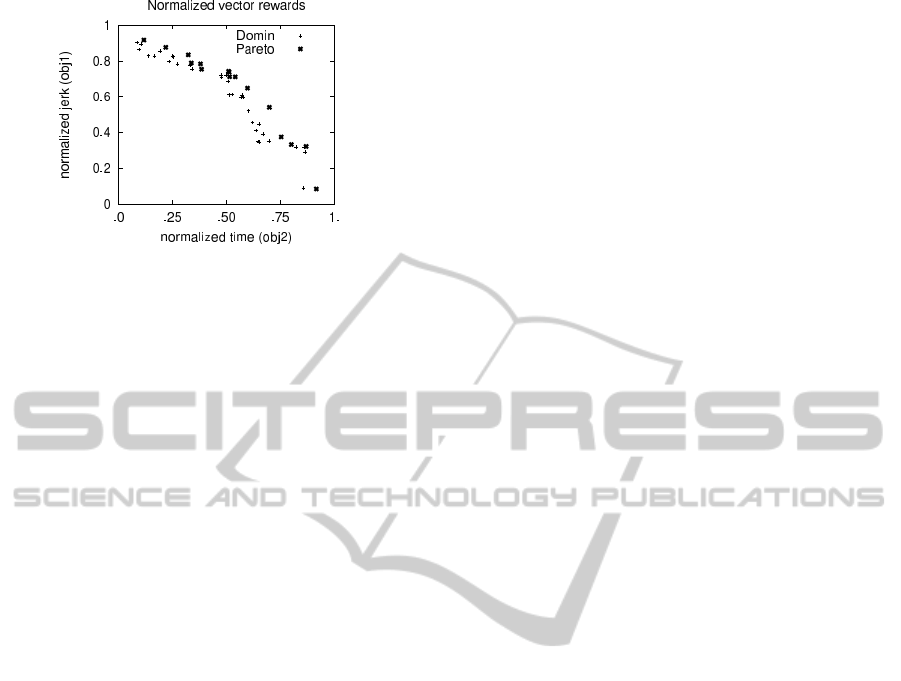
Figure 1: All the points generated by the bi-objective wet-
clutch application.
5 NUMERICAL SIMULATIONS
In this section, we compare the performance of five
Pareto MAB algorithms: 1) a baseline algorithm, 2)
two Pareto UCB1 algorithms and 3) two Pareto UCB2
algorithms. As announced in the introduction, the test
problem is a bi-objective stochastic environment gen-
erated by a real world control application.
The algorithms. The five Pareto MAB algorithms
compared are
tPUCB1. The exploitative Pareto UCB1 algorithm
introduced in Section 3.1;
rPUCB1. The exploratory Pareto UCB1 algorithm
summarised in Section 3.2;
tPUCB2. The exploitative Pareto UCB2 algorithm
summarised in Section 4.1;
rPUCB2. The exploratory Pareto UCB2 algorithm
summarised in Section 4.2;
hoef. A baseline algorithm for multi-armed ban-
dits in general is the Hoeffding race algo-
rithm Maron and Moore (1994) where all the arms
are pulled equally often and the arms with the
non-dominated empirical mean reward vectors are
chosen.
Each algorithm is run 100 times with a fixed
budged, or arm’ pulls, of N = 10
6
. By default, we set
the α parameter for the two Pareto UCB2 algorithms
to 1.
The Wet Clutch Application. In order to optimise
the functioning of the wet clutch Vaerenbergh et al.
(2012) it is necessary to simultaneously minimise 1)
the optimal current profile of the electro-hydraulic
valve that controls the pressure of the oil in the clutch,
and 2) the engagement time. The piston of the clutch
gets in contact with the friction plates to change the
profile of the valve. Such a system is characterised
by a hard non-linearity. Additionally, external fac-
tors that cannot be controlled exactly, e.g. the sur-
rounding temperature, make this a stochastic control
application. Such clutches are typically used in the
power transmission of off-road vehicles that has to
operate under strongly varying environmental condi-
tions. And the goal in this control problem is to min-
imise both the clutch’s profile and the engagement
time under varying environmental conditions.
In Figure 1, we give 54 points generated with the
wet clutch application, each point representing a trial
of the machine and the jerk time obtained in the given
time. The problem was a minimisation problem that
we have transformed into a maximisation problem, by
first normalising each objective with values between
0 and 1, and then transforming it into a maximisation
problem. The best set of incomparable reward vectors
is called the Pareto optimal reward set, i.e. there are
16 such reward vectors. In our example, |A
∗
| is about
one-third from the total number of arms, i.e. 16/54,
and is a mixture of convex and non-convex regions.
In Table 1, we show the mean values of the 54 reward
vectors.
The Performance of the Algorithms. We use four
metrics to measure the performance of the five tested
Pareto MAB algorithms. Two of these metrics are the
Pareto projection regret, cf Equation 2, and the Pareto
variance regret, cf Equation 3, presented in Section 2.
We also use two additional metrics two explain the
dynamics of the Pareto MAB algorithms.
The third metric measures the percentage of times
each Pareto optimal arm is pulled. Thus, for all Pareto
optimal arms, i ∈ A
∗
, we measure E[T
∗
i
(n)] the ex-
pected number of times the arm i is pulled during n
total arm pulls. Note that E[T
∗
i
(n)] is a part of Equa-
tion 3 and it gives a detailed understanding of the
Pareto variance regret.
The last metric is a measure of the running time
of each algorithm, and it is given by the number of
times each arm in A was compared against the other
arms in A in order to compute the Pareto front. Note
that for the exploratory algorithms, i.e. rPUCB1 and
rPUCB2, each arm pull corresponds to one estimation
of the Pareto front, whereas, for the exploitative algo-
rithms, i.e. tPUCB1 and tPUCB2, one estimation of
A
∗
corresponds to the arms’ pulls of the entire set.
5.1 Comparing MOMAB Algorithms
In Figure 2, we compare the performance of the five
MOMAB algorithms. According to the Pareto projec-
tion regret, cf. Figure 2 a), the best performing algo-
rithm is the exploitative Pareto UCB2, cf. tPUCB2,
the second best algorithm is the exploratory Pareto
ExplorationVersusExploitationTrade-offinInfiniteHorizonParetoMulti-armedBanditsAlgorithms
73

Table 1: Fifty-four bi-dimensional reward vectors labelled from 1 to 54 for the wet clutch application. The first sixteen reward
vectors are labeled from µ
∗
1
till µ
∗
16
and are Pareto optimal, while the last thirty-four reward vectors are labelled from µ
17
till
µ
54
and they are suboptimal.
µ
∗
1
= (0.116,0.917) µ
∗
2
= (0.218,0.876) µ
∗
3
= (0.322,0.834) µ
∗
4
= (0.336,0.788)
µ
∗
5
= (0.379,0.783) µ
∗
6
= (0.383,0.753) µ
∗
7
= (0.509,0.742) µ
∗
8
= (0.512,0.737)
µ
∗
9
= (0.514,0.711) µ
∗
10
= (0.540,0.710) µ
∗
11
= (0.597,0.647) µ
∗
12
= (0.698,0.540)
µ
∗
13
= (0.753,0.374) µ
∗
14
= (0.800,0.332) µ
∗
15
= (0.869,0.321) µ
∗
16
= (0.916,0.083)
µ
17
= (0.249,0.826) µ
18
= (0.102,0.892) µ
19
= (0.497,0.722) µ
20
= (0.251,0.824)
µ
21
= (0.249,0.826) µ
22
= (0.102,0.892) µ
23
= (0.497,0.722) µ
24
= (0.251,0.824)
µ
25
= (0.575,0.596) µ
26
= (0.651,0.448) µ
27
= (0.571,0.607) µ
28
= (0.083,0.903)
µ
29
= (0.696,0.350) µ
30
= (0.272,0.784) µ
31
= (0.601,0.521) µ
32
= (0.341,0.753)
µ
33
= (0.507,0.685) µ
34
= (0.526,0.611) µ
35
= (0.189,0.857) µ
36
= (0.620,0.454)
µ
37
= (0.859,0.314) µ
38
= (0.668,0.388) µ
39
= (0.334,0.782) µ
40
= (0.864,0.290)
µ
41
= (0.473,0.722) µ
42
= (0.822,0.316) µ
43
= (0.092,0.863) µ
44
= (0.234,0.796)
µ
45
= (0.476,0.709) µ
46
= (0.566,0.596) µ
47
= (0.166,0.825) µ
48
= (0.646,0.349)
µ
49
= (0.137,0.829) µ
50
= (0.511,0.611) µ
51
= (0.637,0.410) µ
52
= (0.329,0.778)
µ
53
= (0.649,0.347) µ
54
= (0.857,0.088)
UCB2, cf rPUCB2, and the worst algorithm is the
Hoeffding race algorithm, cf. hoef. Note that the
Pareto UCB1 family of algorithms has a (almost) lin-
ear regret whereas Pareto UCB2 algorithms have a
logarithmic regret, like the single objective UCB2 al-
gorithm. The worst performance of the exploitative
Pareto UCB1 algorithm can be explained by the poor
explorative behaviour of the algorithm. The perfor-
mance of the explorative Pareto UCB1 is in-between
linear and logarithmic and can be explained by the im-
proved exploratory technique of pulling all the Pareto
optimal arms each round. Both Pareto UCB2 algo-
rithms perform better than Pareto UCB1 algorithms
because the Pareto optimal arms are explored longer
each round.
In opposition, according to the Pareto variance re-
gret, cf. Figure 2 b), the worst performing algorithms
are the exploitative and exploratory Pareto UCB2 al-
gorithms and the best algorithms are the exploratory
and exploitative Pareto UCB1 algorithms but also the
Hoeffding race algorithm. It is interesting to note that
the difference in Pareto variance and projection re-
gret between the exploratory and exploitative variance
of the same algorithms is small. In general, Pareto
UCB1 algorithms have a larger Pareto projection re-
gret then the Pareto UCB2 algorithms, but a smaller
Pareto variance regret.
Figure 2 c) explains these contradictory results
with the percentage of times each of the Pareto op-
timal arms are pulled. As noticed in Section 4.2, the
exploratory Pareto UCB2, cf rPUCB2, pulls the same
Pareto optimal arm each epoch longer and longer,
generating the peak in the figure on one random sin-
gle Pareto optimal arm. In contrast, the exploitative
Pareto UCB2, cf. tPUCB2, is fair in exploiting the
entire Pareto front. In the sequel, the exploratory
Pareto UCB1 algorithm, cf rPUCB1, has more vari-
ance in pulling Pareto optimal arms than the exploita-
tive Pareto UCB2 algorithm, cf tPUCB1, and this fact
is reflected also in the Pareto variance regret measures
from Figure 2 b).
The percentage of time of the any Pareto optimal
arms is pulled: 1) for the exploitative Pareto UCB2
is 83% ±8.5, 2) for the explorative Pareto UCB2 is
77% ±10.9, 3) for the exploitative Pareto UCB1 is
49%±4.9, and 4) for the explorative UCB1 is 49%±
4.9. Note the large difference between the efficiency
of Pareto UCB2 and Pareto UCB1 algorithms.
In Figure 2 d), we show that the running time,
i.e. number of comparisons between arms, for ex-
ploratory MOMABs, i.e. the exploratory Pareto
UCB1 and the exploratory Pareto UCB2, are order of
magnitude larger than the exploitative MOMAB algo-
rithms, i.e. the exploitative Pareto UCB1 and the ex-
ploitative Pareto UCB2. The running time for Pareto
UCB1 algorithms which compute the Pareto front of-
ten is larger than the running time for Pareto UCB2
algorithms that compute the Pareto front once in the
beginning of an epoch. The most computational ef-
ficient is the exploitative Pareto UCB2 and the worst
algorithm is the exploratory Pareto UCB1.
5.2 Exploration vs Exploitation
Mechanism in Pareto UCB2
Algorithms
In our second experiment, we measure the influence
of the parameter α on the performance of Pareto
UCB2 algorithms. Figure 3 considers five values for
this parameter α = {0.1, 0.5,1.0,2.0,4.0} that indi-
cates the length of an epoch. The largest variance
in performance we have for the exploratory Pareto
ICAART2015-InternationalConferenceonAgentsandArtificialIntelligence
74
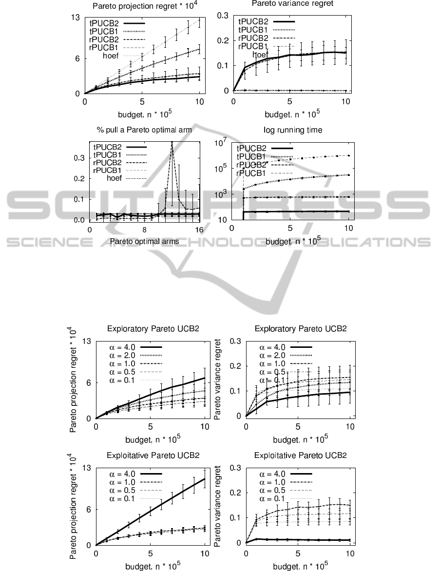
(a) (b)
(c) (d)
Figure 2: The performance of the five MOMAB algorithms on the wet clutch problem: a) the Pareto projection regret, b)
the Pareto variance regret, c) the percentage of times each Pareto optimal arm is pulled, and d) the running time in terms of
comparisons between arms and Pareto front for each MOMAB algorithm. The five algorithms are: 1) tPUCB1 the exploitative
Pareto UCB1, 2) rPUCB1 the exploratory Pareto UCB1, 3) tPUCB2 the exploitative Pareto UCB2, 4) rPUCB2 the exploratory
Pareto UCB2, and 5) hoef the Hoeffding race algorithm.
(a) (b)
(c) (d)
Figure 3: The performance of the two version of Pareto UCB2 algorithms, i.e. exploratory and exploitative Pareto UCB2,
given for the five values of the α = {0.1,0.5, 1.0,2.0, 4.0} parameter.
ExplorationVersusExploitationTrade-offinInfiniteHorizonParetoMulti-armedBanditsAlgorithms
75
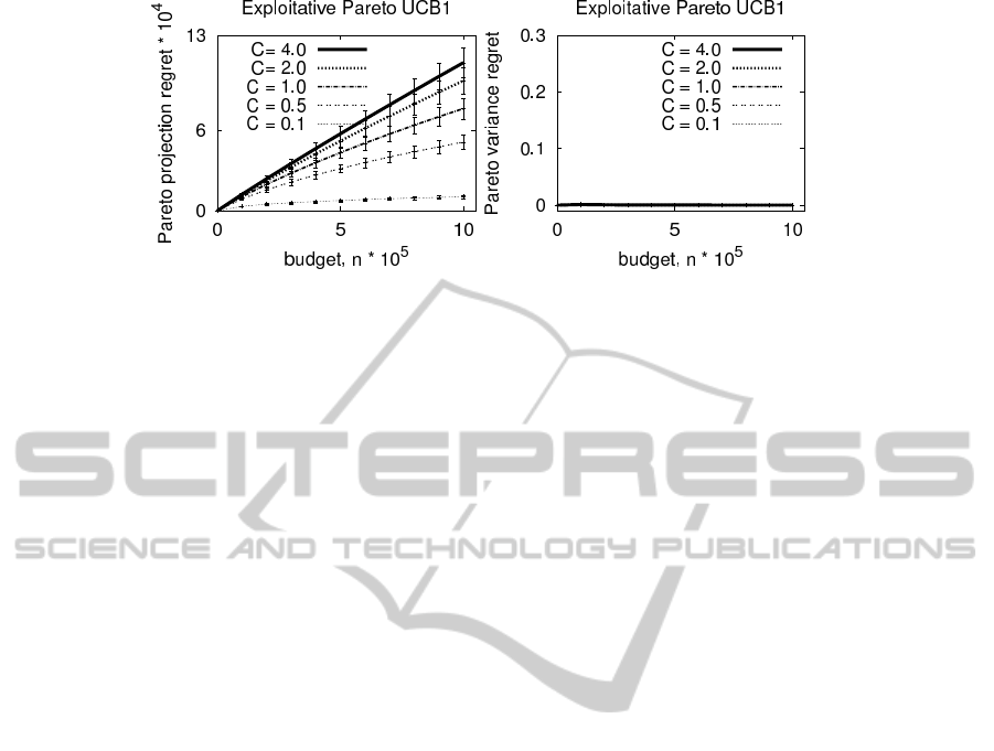
(a) (b)
Figure 4: The performance of the exploitative Pareto UCB1 algorithm given five values of the C = {0.1,0.5,1.0, 2.0,4.0}
parameter multiplying the index value.
UCB2. The smaller is the size of an epoch, the bet-
ter the performance of the exploratory Pareto UCB2
algorithm is in terms of Pareto projection regret and
Pareto variance regret. Note that for epochs’ length
of 1, the Pareto UCB2 algorithms resemble the Pareto
UCB1 algorithms, meaning that an arm or a set of
arms are pulled each epoch. Of course, the two algo-
rithms have a different exploration index. The same
parameter α has little influence on the performance
of exploitative Pareto UCB2 algorithm where all the
Pareto arms are pulled each epoch.
5.3 Exploration vs Exploitation
Trade-off in Pareto UCB1
Algorithms
To study the influence of the exploration index for the
Pareto UCB1 algorithm, we multiply the index of ex-
ploitative Pareto UCB1 with a constant C that takes
five values C = {0.1,0.5, 1.0,2.0,4.0}. Unlike for
the exploitative Pareto UCB2 algorithm, the constant
C has a big influence on the performance of Pareto
UCB1 algorithms. The smaller is the multiplication
constant, the better is the performance of the exploita-
tive Pareto UCB1 algorithm. This means that an ex-
ploitative Pareto UCB1 algorithm performs the best
with a small exploration index.
6 CONCLUSION
In this paper, we investigate the exploration vs ex-
ploitation trade-off in two of the infinite horizon
MABs. The classical UCB1 and UCB2 algorithms
are extended to reward vectors those quality is classi-
fied with Pareto dominance relation. We analytically
and experimentally study the regret, i.e. the Pareto
projection regret and the Pareto variance regret, of the
proposed MOMAB algorithms.
We propose the exploitative Pareto UCB1 algo-
rithm that each round pulls all the Pareto optimal
arms. The exploratory version of the same algorithm
uniform at random selects each round only one arm
Pareto optimal arm. We show that this difference has
an important impact on the upper Pareto projection
regret bound of the exploitative Pareto UCB1 algo-
rithm. Now, the upper regret bound is independent of
the cardinality of the Pareto front, which is large for
many objective environments, and, furthermore, un-
known beforehand.
Based on the same principle, we propose the ex-
ploratory and exploitative Pareto UCB2 algorithms.
The exploratory Pareto UCB2 algorithm pulls each
epoch a single Pareto optimal arm selected at ran-
dom. The exploitative Pareto UCB2 pulls, each
epoch, equally often all the Pareto optimal arms. We
upper bound the Pareto projection regret of the ex-
ploitative Pareto UCB2 algorithm.
We compare these algorithms also experimentally
on a bi-objective problem coming from control the-
ory. Our conclusion is that the exploration vs ex-
ploitation trade-off is better in the exploitative Pareto
algorithms where all the Pareto optimal arms are
pulled often. In opposition, the exploratory Pareto
UCB2 algorithm has a small Pareto projective vari-
ance regret but a large Pareto variance regret since the
algorithm pulls a single Pareto optimal arm during ex-
ponentially large epochs.
REFERENCES
Auer, P., Cesa-Bianchi, N., and Fischer, P. (2002). Finite
time analysis of the multiarmed bandit problem. Ma-
chine Learning, 47(2/3):235–256.
Drugan, M. and Nowe, A. (2013). Designing multi-
objective multi-armed bandits: a study. In Proc of
ICAART2015-InternationalConferenceonAgentsandArtificialIntelligence
76

International Joint Conference of Neural Networks
(IJCNN).
Lizotte, D., Bowling, M., and Murphy, S. (2010). Efficient
reinforcement learning with multiple reward functions
for randomized clinical trial analysis. In Proceed-
ings of the Twenty-Seventh International Conference
on Machine Learning (ICML).
Maron, O. and Moore, A. (1994). Hoeffding races: Accel-
erating model selection search for classification and
function approximation. In Advances in Neural Infor-
mation Processing Systems, volume 6, pages 59–66.
Morgan Kaufmann.
Vaerenbergh, K. V., Rodriguez, A., Gagliolo, M., Vrancx,
P., Nowe, A., Stoev, J., Goossens, S., Pinte, G., and
Symens, W. (2012). Improving wet clutch engage-
ment with reinforcement learning. In International
Joint Conference on Neural Networks (IJCNN). IEEE.
van Moffaert, K., Drugan, M., and Nowe, A. (2013).
Hypervolume-based multi-objective reinforcement
learning. In Proc of Evolutionary Multi-objective Op-
timization (EMO). Springer.
Wang, W. and Sebag, M. (2012). Multi-objective Monte
Carlo tree search. In Asian conference on Machine
Learning, pages 1–16.
Wiering, M. and de Jong, E. (2007). Computing optimal sta-
tionary policies for multi-objective markov decision
processes. In Proc of Approximate Dynamic Program-
ming and Reinforcement Learning (ADPRL), pages
158–165. IEEE.
Zitzler, E., Thiele, L., Laumanns, M., Fonseca, C. M., and
da Fonseca, V. (2003). Performance assessment of
multiobjective optimizers: An analysis and review.
IEEE T. on Evol. Comput., 7:117–132.
ExplorationVersusExploitationTrade-offinInfiniteHorizonParetoMulti-armedBanditsAlgorithms
77
