AGAGD
An Adaptive Genetic Algorithm Guided by Decomposition for Solving PCSPs
Lamia Sadeg-Belkacem
1,2,3
, Zineb Habbas
2
and Wassila Aggoune-Mtalaa
4
1
Ecole Nationale Superieure d’Informatique, Algiers, Algeria
2
LCOMS, University of Lorraine, Ile du Saulcy, 57045 Metz Cedex, France
3
Laboratory of Applied Mathematics, Military Polytechnic School, Algiers, Algeria
4
Public Research Centre Henri Tudor, Luxembourg, G.D. Luxembourg
Keywords:
Optimization Problems, Partial Constraint Satisfaction Problems, Graph Decomposition, Adaptive Genetic
Algorithm (AGA), AGA Guided by Decomposition.
Abstract:
Solving a Partial Constraint Satisfaction Problem consists in assigning values to all the variables of theproblem
such that a maximal subset of the constraints is satisfied. An efficient algorithm for large instances of such
problems which are NP-hard does not exist yet. Decomposition methods enable to detect and exploit some
crucial structures of the problems like the clusters, or the cuts, and then apply that knowledge to solve the
problem. This knowledge can be explored by solving the different sub-problems separately before combining
all the partial solutions in order to obtain a global one. This was the focus of a previous work which led to
some generic algorithms based on decomposition and using an adaptive genetic algorithm, for solving the
subproblems induced by the crucial structures coming from the decomposition.
This paper aims to explore the decomposition differently. Indeed, here the knowledge is used to improve this
adaptive genetic algorithm. A new adaptive genetic algorithm guided by structural knowledge is proposed. It
is designed to be generic in order that any decomposition method can be used and different heuristics for the
genetic operators are possible. To prove the effectiveness of this approach, three heuristics for the crossover
step are investigated.
1 INTRODUCTION
A Partial Constraint Satisfaction Problem (PCSP) is
a partial version of a CSP for which only a subset
of constraints called hard constraints have to be sat-
isfied. The rest of the constraints of the problem
called soft constraints can be violated in the condi-
tion that a penalty is involved. In other words, PC-
SPs are CSPs for which penalties are assigned to soft
constraints that are not satisfied. When addressing
a PCSP, the objective is to assign values to all vari-
ables such as to minimize the total penalty, also called
the cost of the solution, induced by the violated con-
straints. A large class of Problems can be modeled
as a PCSP including for example Maximum Satisfi-
ability Problems, Boolean Quadratic Problems (Tate
and Smith, 1995) or Coloring Problems (Zhou et al.,
2014). In this paper, the Frequency Assignment Prob-
lem (FAP), one of the most well known combinato-
rial Problems, is taken as experimental target to val-
idate our approach. Indeed, the focus of this work
is on binary PCSPs where any constraint involves
two variables. When looking for a global solution
of the PCSP, generic solvers are sometimes surpris-
ingly competitive but other times, these solvers re-
ally fail to address large size problems because of
some difficult subproblems that lurk beneath. PC-
SPs (and particularly FAPs) have been solved by a
number of different exact approaches (enumerative
search, Branch & Bound for instance) and numer-
ous heuristics or metaheuristics (Maniezzo and Car-
bonaro, 2000; Kolen, 2007; Voudouris and Tsang,
1995). However all these approaches have often a
limited success when coping with real large instances.
Nowadays solving approaches propose to explore the
structure of the associated constraint graph (Allouche
et al., 2010; Colombo and Allen, 2007). In particular,
methods exploiting tree decompositions (Koster et al.,
2002) are known to be among the best techniques
with regard to theoretical time complexity. Unfor-
tunately these methods have not shown a real effi-
ciency for large problems thus proving a practical in-
78
Sadeg-Belkacem L., Habbas Z. and Aggoune-Mtalaa W..
AGAGD - An Adaptive Genetic Algorithm Guided by Decomposition for Solving PCSPs.
DOI: 10.5220/0005196400780089
In Proceedings of the International Conference on Agents and Artificial Intelligence (ICAART-2015), pages 78-89
ISBN: 978-989-758-074-1
Copyright
c
 2015 SCITEPRESS (Science and Technology Publications, Lda.)

terest. In (Sadeg-Belkacem et al., 2014), a generic ap-
proach based on decomposition was introduced. This
aim is to solve large size problems in a short time
but not necessarily at optimality. This approach uses
Multicut Decompositions for decomposing the PCSP,
which consists in splitting the weighted graph asso-
ciated with the PCSP into k subgraphs connected by
a set of constraints which constitutes the multicut.
This decomposition step induces different strategies
for the solving algorithm. Several solving variants
have been studied and experimented on well known
FAP benchmarks. The computational results, using
an Adapative Genetic Algorithm (AGA) for solving
the subproblems are relatively promising. In this pa-
per, the new idea is to exploit structural knowledges
coming from the decomposition method in an inno-
vative way. A recent study has shown the benefits
of such an approach for improving a local search
method (Fontaine et al., 2013; Loudni et al., 2012;
Ouali et al., 2014). In particular, the tree decom-
position was explored. In this work, the approach
is more generic since any decomposition can be ex-
plored. Therefore, a new generic algorithm is pro-
posed. It is called AGAGD
x y for Adaptive Genetic
Algorithm Guided by Decomposition. AGAGD x y
uses a given decomposition method to detect crucial
substructures of the problem and then applies that
knowledge to boost the performance of the AGA it-
self. The name of the algorithm is indexed by x and
y, where x is for the generic decomposition and y is
for the generic genetic operator. In this paper three
heuristics named Crossover
clus, Crossover cut and
Crossover clus cut are presented.
The paper is organized as follows. Section 2 gives
a formal definition of a PCSP. Section 3 presents
the decomposition method chosen to validate this ap-
proach. In section 4 an efficient Adaptive Genetic Al-
gorithm for solving PCSPs is proposed. The proposi-
tion of an Adaptive Genetic Algorithm Guided by De-
composition AGAGD
x y is presented in section 5.
The first computational and promising results are pre-
sented in section 6. The paper ends with a conclusion
and perspectives for further research.
2 PARTIAL CONSTRAINT
SATISFACTION PROBLEM
(PCSP)
Definition 1 (Constraint Satisfaction Problem). A
Constraint Satisfaction Problem (CSP) is defined as
a triple P =< X,D,C > where
• X = {x
1
,...,x
n
} is a finite set of n variables.
• D = {D
1
,...,D
n
} is a set of n finite domains. Each
variable x
i
takes its value in the domain D
i
.
• C = {c
1
,...,c
m
} is a set of m constraints. Each
constraint c
i
is defined as a set of variables
{x
i
,... ,x
j
}, i, j = 1,... ,n called the scope of c
i
.
For each constraint c
i
a relation R
i
specifies the
authorized values for the variables. This relation
R
i
can be defined as a formula or as a set of tuples,
R
i
⊆
∏
(x
k
∈c
i
)
D
k
(subset of the cartesian product).
A solution of a CSP is a complete assignment of
values to each variable x
i
∈ X denoted by a vector
< d
1
,d
2
,... ,d
n
> (where d
i
∈ D
i
∀i ∈ 1...n) which
satisfies all the constraints of C.
Remark 1. The cardinality of c
i
is called the arity
of constraint c
i
. CSPs with constraints involving at
most two variables are named binary CSPs.
Let us recall that in this work, only binary CSPs are
considered. In the rest of the paper, a constraint
c = {x
i
,x
j
} is denoted by (x
i
,x
j
).
Definition 2 (Binary Partial Constraint Satisfaction
Problem). A binary Partial Constraint Satisfaction
Problem is defined as a quadruplet P =< X, D,C,P >
where
• < X,D,C > is a binary CSP,
• P = {p
1
,..., p
m
} is a set of m penalties. Each
penalty p
i
is a value associated with a constraint
c
i
, i = 1,... ,m.
The objective when solving a PCSP is to select an au-
thorized value for each variable x
i
∈ X such that the
sum of the penalties of the violated constraints called
also the cost of the solution s and defined as follows:
cost(s) =
m
∑
i=1
p
i
where c
i
is violated
has to be minimized.
Definition 3 (Constraint Graph). Let P =<
X,D,C, P > be a PCSP. Let G = (V,E) be the
undirected weighted graph associated with P as
follows: with each variable x ∈ X we associate a
node v
x
∈ V and for each constraint (x
1
,x
2
) ∈ C we
define an edge v
x
1
v
x
2
∈ E and a weight w associated
with its penalty defined in P.
Remark 2. Among the set of constraints, those that
must not be violated are called ”hard” constraints
while the others are ”soft” constraints.
AGAGD-AnAdaptiveGeneticAlgorithmGuidedbyDecompositionforSolvingPCSPs
79

3 DECOMPOSITION
TECHNIQUES
3.1 Generalities on Decomposition
Techniques
The objective of a decomposition method is to split
a large problem into a collection of interconnected
but easier sub-problems. The decomposition tech-
niques can generally be applied to various problems.
Therefore, a huge strand of research is dedicated to
decomposition techniques. The decomposition pro-
cess depends on the nature of the problem and how
it is modelled (Schaeffer, 2007). In this study, the
focus is on decomposition techniques which include
graph decompositions such as graph partitioning or
graph clustering particularly adapted to optimization
problems which are modelled by graphs.
This section uses interchangeably the terms cluster-
ing and partitioning and proposes methods to built a
k-partition {C
1
,C
2
,... ,C
k
} of a given weighted graph
G =< V,E >. The clusters of the partition have no
shared variable and they are connected by a set of
edges. The end of such edges constitute the cut of
the decomposition. Building such a k-partition can
be done in many ways. Each method depends on
the expected structure for the clusters, the expected
properties for the cut and on the main goal of the
resulting partition. Moreover decomposition tech-
niques can be global or local (Schaeffer, 2007). Local
decompositions have been discarded in this study
because they assign a cluster for only some variables
of the problem, while in global decomposition
methods, each variable is assigned to one cluster of
the resulting partition.
The approach proposed in this paper is completely
generic. It is not conditioned by any particular de-
composition method. Therefore the performance of
the approach has to be assessed by considering sev-
eral decomposition methods with different properties.
However as the aim of this first work is rather to vali-
date the new AGAGD
x y algorithm, the well known
powerful clustering algorithm due to Newman (New-
man, 2004) is considered as target decomposition
method.
3.2 Newman Algorithm
In recent years, with the development of the web
research, many clustering algorithms for data min-
ing, information retrieval or knowledge mining have
been proposed. A common property that summa-
rizes all these algorithms is the community structure:
the nodes of the networks are grouped into clusters
with a high internal density and clusters are sparsely
connected. To detect structure communities in net-
works, an algorithm based on an iterative removal of
edges is proposed in (Girvan and Newman, 2002).
The main drawback of this algorithm is its compu-
tational time. Indeed, its worst case time complex-
ity is in O(m × n
2
) on a network with m edges and
n nodes or O(n
3
) on a sparse graph. This limits the
use of this algorithm to problems with a few thousand
nodes at most. A more efficient algorithm for detect-
ing community structure is presented in (Newman,
2004), with a worst time complexity in O((m+n)×n)
or O(n
2
) on a sparse graph. In practice, this algorithm
runs on current computers in a reasonable time for
networks of up to a million vertices, so the instances
considered previously are intractable. The principle
of this new algorithm (denoted Newman algorithm) is
based on the idea of modularity. The first algorithm
presented in (Girvan and Newman, 2002), (Newman,
2004) splits the network into communities, regardless
of whether the network has naturally such a division.
To define the meaningfulness of a decomposition, a
quality function denoted Q or modularity is associ-
ated. Given a network G =< V,E >, let e
ij
be the
fraction of edges in G that connects the nodes in clus-
ter i to those in cluster j and let a
i
=
∑
j
e
ij
, then
Q =
∑
i
(e
ii
− a
2
i
)
In practice, values of Q greater than about 0,3 give a
significant community structure. In (Newman, 2004),
an alternative approach is suggested to find commu-
nity structures: Q is simply optimized instead of con-
sidering different iterative removals of edges. How-
ever the optimization of Q is very expensive. In prac-
tice, looking for all possible divisions for optimizing
Q takes at least an exponential amount of time and it
is infeasible for networks larger than 20 or 30 nodes.
Different heuristic or metaheuristic algorithms can be
used to approximate this problem.
Newman uses an iterative agglomerative algorithm
that is a bottom-up hierarchical one. This algorithm
starts by considering n clusters or n communities, for
which each community contains only one node. The
communities are then repeatedly joined in pairs. The
algorithm chooses at each step the join that results
in the smallest decrease of Q. The algorithm pro-
gresses like a dendrogram at different nodes. The cuts
through this dendrogram at different levels give the
divisions of the graph into a certain number of com-
munities of different sizes. The best cut is chosen by
looking for the maximal value for Q. This new ver-
sion of the algorithm is in O(n
2
) on sparse graphs.
ICAART2015-InternationalConferenceonAgentsandArtificialIntelligence
80

3.3 Detected Structural Knowledge
This subsection is dedicated to the presentation of
general concepts linked with decomposition tech-
niques. These concepts will be used in the rest of
the paper and will facilitate the presentation of the
AGAGD x y algorithm.
Definition 4 (Partition, Cluster). Given a graph
G =< V,E >, a partition {C
1
,C
2
,... ,C
k
} of G is a
collection of subsets of V that satisfies the following:
•
k
S
i=1
C
i
= V
• ∀i, j = 1,. . .,k : C
i
∩C
j
=
/
0
Each subset of variables C
i
of the partition of G is
called a cluster.
Definition 5 (Cut). Let {C
1
,C
2
,... ,C
k
} be a partition
of a graph G =< V, E >, and let C
i
and C
j
be two
clusters. We denote by Cut(C
i
,C
j
) the set of vertices
{u ∈ V
i
,∃v ∈ V
j
and uv ∈ E} ∪ {v ∈ V
j
,∃u ∈ V
i
and
uv ∈ E}.
Definition 6 (Separator). Let G =< V, E > be a
graph and P = {C
1
,C
2
,... ,C
k
} a partition of this
graph. Let C
i
be a cluster in P. The separator of
C
i
denoted Sep(C
i
) is the set of vertices defined by:
Sep(C
i
) = {u ∈ V
i
,∃v /∈ V
i
and uv ∈ E}. In other
words, Sep(C
i
) is the set of the bordering nodes of C
i
.
Remark 3. Let P = < X,D,C, P > be a PCSP and G
= < V,E > its weighted graph representation where
V = X , E = C and |V| = n. In the rest of this paper
G[V
S
] will denote the subgraph < V
S
,E
S
> induced
by the subset of nodes V
S
in V.
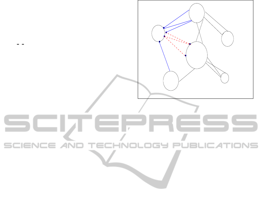
Example 1. This small example illustrates the impor-
tant concepts related to structural knowledge.
Figure 1 presents a constraint graph decomposed
into a partition {C
1
,C
2
,C
3
,C
4
,C
5
,C
6
} of 6 clus-
ters, where Cut(C
1
,C
5
) = {b,c,e, f} and Sep(C
1
) =
{a,b, c,d}.
4 ADAPTIVE GENETIC
ALGORITHM FOR PCSPs
(AGA)
4.1 Motivation
This section presents an Adaptive Genetic Algorithm
C6
C3
C2
C1
C4
f
e
a
b
c
d
C5
Figure 1: Example of sep and cut notions.
(AGA) specific to PCSPs. Genetic algorithms are the
most popular heuristics used for optimization prob-
lems. Several variants of GA for solving PCSPs have
been proposed in the literature. Thus the proposition
of a new genetic algorithm does not constitute the
major contribution of this paper. However, building
an effective GA is a first step to validate the practical
benefit of this present approach. A GA involves some
parameters which should be adjusted in order to
provide good results. A judicious choice of crossover
and mutation probabilities is crucial for improv-
ing its performance. Indeed, a standard genetic
algorithm cannot find the optimum in a reasonable
time (Lee and Fan, 2002). This is mainly due to the
fact that crossover and mutation probabilities are
predetermined and fixed. The population becomes
premature and falls in local convergence early. To
avoid this drawback an Adaptive Genetic Algorithm
(AGA) is proposed, in which mutation and crossover
probabilities change during the execution process, in
order to improve the exploration of the search space.
4.2 Useful Definitions
The following definitions are introduced for the sake
of clarity in the presentation of the AGA.
Definition 7 (Neighborhood). Let P = < X,D,C,P >
be a PCSP and G = < V,E > its weighted constraint
graph. The neighborhood of the vertex v
i
in G is
defined by : N[v
i
] = {v
j
∈ V|(v
i
,v
j
) ∈ E}.
Definition 8 (Chromosome). Let P = < X, D,C,P >
be a PCSP. A chromosome s is a mapping of a n-tuple
of variables (x
1
,x
2
,... ,x
n
) → D
1
× D
2
× . .. × D
n
which assigns to each variable in X a value of its
AGAGD-AnAdaptiveGeneticAlgorithmGuidedbyDecompositionforSolvingPCSPs
81

corresponding domain.
Definition 9 (Feasible Solution). Let P =
< X,D,C,P > be a PCSP. A feasible solution s
of P is a chromosome s = (s
1
,s
2
,... ,s
n
) where
s
i
∈ D
i
∀i = 1,..n, that satisfies all the hard con-
straints.
Definition 10 (Population). A population P is a set
of chromosomes.
Definition 11 (Gene). Each component s
i
of the
chromosome s = (s
1
,s
2
,... ,s
n
), i = 1,.., n, is called a
gene.
Definition 12 (Fitness of a gene). Let P =
< X, D,C,P > be a PCSP and G = < V, E > its
weighted constraint graph. The fitness of the gene
s
i
in the chromosome s is defined by: Fitness (s
i
,s)
=
∑
v
j
∈N[v
i
],(v
i
,v
j
)∈unsat
w(v
i
,v
j
).(unsat is for the con-
straints which are not satisfied).
Definition 13 (Fitness of a Chromosome). The
fitness of the chromosome s = (s
1
,... ,s
n
) is defined
by: Fitness (s) =
1
2
n
∑
i=1
Fitness(s
i
,s).
4.3 Presentation of the Adaptive
Genetic Algorithm (AGA) for
PCSPs
Notations
• p
m
0
: initial mutation probability
• p
c
0
: initial crossover probability
• p
m
min
: mutation probability threshold
• p
c
max
: crossover probability threshold
• ∆p
m
: mutation probability rate
• ∆p
c
: crossover probability rate
To solve a problem with a genetic algorithm, the
first step that is crucial is to define a representation of
the problem state.
An initial population is then defined and is submitted
to the two genetic operations mutation and crossover.
This enables to generate the next generation. This
procedure is repeated until a convergence criterion is
reached. AGA is formally given by Algorithm 1.
Algorithm 1: AGA(Pb: a PCSP, s: a solution).
Input:G < V,E,W >: constraint graph for a PCSP,
p
m
0
, p
c
0
, p
m
min
, p
c
max
, ∆p
m
, ∆p
c
, nb: mutation pa-
rameter
1: p ← Initial
Population;
2: if local mimima
1
then
3: p
m
← p
m
− ∆p
m
4: p
c
← p
c
+ ∆p
c
5: if p
m
< p
m
min
then
6: p
m
← p
m
min
7: end if
8: if p
c
> p
c
max
then
9: p
c
← p
c
max
10: end if
11: else
12: p
m
← p
m
0
13: p
c
← p
c
0
14: end if
15: old
p ← p
16: repeat
17: for all i=1 to size(old
p) do
18: in parallel
19: parent
i ← the ith chromosome in old p
20: parent j ← the selected chromosome in
old
p using the tournament algorithm
21: if p
c
ok then
22: offspring
i ← Crossover(parent i, par-
ent j), where offspring i will be the ith
chromosome in a future population.
23: else
24: offspring
i ← parent i
25: end if
26: if p
m
ok then
27: offspring
i ← Mutation(offspring i, nb)
28: end if
29: end for
30: until convergence
The performance of AGA is tightly dependent on
its crossover and mutation operators. The mutation
operator is used to replace the values of a certain num-
ber of genes, randomly chosen in the parent popula-
tion, in order to improve the fitness of the resulting
chromosome. The mutation occurs with a probability
p
m
, named mutation probability. The crossover oper-
ation is used to generate a new offspring by exchang-
ing the values of some genes, to improve the fitness
of a part of the chromosome. A crossover appears
only with a probability p
c
called the crossover proba-
bility. p
m
and p
c
are two complementary parameters
1
The local minima considered in this algorithm corre-
sponds to the minimum cost in the population obtained suc-
cessively a certain number of times.
ICAART2015-InternationalConferenceonAgentsandArtificialIntelligence
82

which have to be fine tuned. Indeed a good value for
p
c
avoids the local optima (diversification) while p
m
enables the GA to improve the quality of the solutions
(intensification).
In the proposed AGA, both parameters are dynami-
cally modified to reach a good balance between the
intensification and the diversification. More precisely,
the crossover (respectively the mutation) operator is
called each time p
c
(respectively p
m
) reaches a certain
threshold, setting the Boolean value p
c
ok (respec-
tively p
m
ok) to true. These probabilities are never-
theless bounded by p
m
min
and p
c
max
, to avoid too much
disruption in the population, which slows the conver-
gence of the algorithm. Since all chromosomes of a
given population are independent, crossover and mu-
tation operations are processed concurrently.
4.3.1 Crossover in AGA
The crossover operator (Algorithm 2) aims to mod-
ify the solution while reducing the degradation of its
cost. It consists in replacing, in the current solution,
the elements and their neighborhoodwhich have a bad
fitness by ones which have a fitness of good quality in
an individual selected by the tournament method (Al-
gorithm 1).
Algorithm 2: Crossover(p
1
, p
2
).
1: New Fitness[p
1
] ← Fitness[p
1
]
2: New
Fitness[p
2
] ← Fitness[p
2
]
3: for all i = 1 to n do
4: New
Fitness[p
1
](i) ← New Fitness[p
1
](i)+
∑
v
j
∈N[v
i
]
Fitness[p
1
]( j)
5: New
Fitness[p
2
](i) ← New Fitness[p
2
](i)+
∑
v
j
∈N[v
i
]
Fitness[p
2
]( j)
6: end for
7: Temp ← New
Fitness[p
1
] -New Fitness[p
2
]
8: Let j = k such that Temp[k] is the largest element
in Temp.
9: for all i = 1 to n do
10:
of fspring[i] ←

p
1
[i] ifi 6= jand v
i
/∈ N[v
j
]
p
2
[i] otherwise
11: end for
4.3.2 Mutation in AGA
Contrarily to the mutation in a classical genetic algo-
rithm which objective is to perturb the solution, the
mutation operator in AGA aims at enhancing the so-
lution cost. Indeed, as presented in (Algorithm 3), this
new mutation applies the local search method 1 opt to
several elements of the solution (randomly chosen),
until it is no more possible to enhance the cost during
a certain number of successive iterations. The aim of
this operation is twofold. First, it aims to enhance the
quality of the population, for a large number of off-
springs. Second, in the case where the solution 1
opt
of a good quality solution is optimum, the solution
has to converge to optimality.
Algorithm 3: Mutation(s,nb).
1: best ← 0
2: while best < nb do
3: select an element s
i
from s
1
4: new
s ← s
5: 1 opt(new s, si)
6: if Fitness[new
s] < Fitness[s] then
7: new s ← s
8: nb ← 0
9: else
10: best++
11: end if
12: end while
13: s ← New
s
5 ADAPTIVE GENETIC
ALGORITHM GUIDED BY
DECOMPOSITION: AGAGD
x y
5.1 Presentation of AGAGD
This section aims to present the new AGAGD
x y al-
gorithm. The formal description of AGAGD x y is
given by Algorithm 4.
Algorithm 4: AGAGD x y (Pb: a PCSP, s: a solution).
1: Input: G = < V,E > is a weighted constraint
graph associated with Pb
2: Decompose
x(G, C = {C
1
,... ,C
k
})
3: AGA
y(Pb, C, s )
This algorithm consists of two major steps, as fol-
lows:
• The first step (Procedure Decompose) parti-
tions the constraint network corresponding to
the initial problem Pb to be solved in order
to identify some relevant structural compo-
nents such that clusters, cuts, or separators for
instance. The multicut decomposition method
1
Depending on a given probability, s
i
is either chosen
randomly or those presenting the maximum fitness
AGAGD-AnAdaptiveGeneticAlgorithmGuidedbyDecompositionforSolvingPCSPs
83

used in this paper has been presented in section 3.
• The second step of the algorithm is related to the
algorithm AGA
y. The algorithm is indexed by y,
meaning that it is generic and that several variants
can be considered. Indeed, the most repetitive
important operation in a genetic algorithm is
the crossover one. In AGA, this operation
involves at each time, a unique variable and its
neighborhood. That explains why the number
of the crossover steps needed can be very high
before obtaining a convergence state. In order
to boost the AGA, the algorithm AGA
y will
exploit structural knowledge coming from a given
multicut decomposition. More specifically, rather
than operating a crossover on a single variable at
each step, it applies it on more crucial parts of the
problems, such that clusters, cuts, separators or
any other relevant structural knowledge. Formally
the algorithm AGA
y corresponds to AGA for
which the crossover procedure is replaced by
crossover
y.
It is clear that several versions of crossover
y can be
studied. In the present work, three different heuristics
are introduced as described further.
5.2 Definition
Definition 14 (Fitness of a cluster). Given a PCSP
P = < X, D,C,P > , its weighted constraint graph
G =< V,E > and a partition P = {C
1
,C
2
,... ,C
k
} of
G. Let s be a current solution of P and C
i
a cluster
in P. Let us consider G
i
[C
i
] =< V
i
,E
i
> the subgraph
induced by C
i
in G. The fitness of the cluster C
i
is
defined by:
Fitness[C
i
,s] =
∑
(v
i
,v
j
)∈E
i
w(v
i
,v
j
)
where (v
i
,v
j
) ∈ E
i
and (v
i
,v
j
) is unsatisfied in s.
Remark 4. To obtain the definition of the fitness of a
cut, one should replace the word cluster by the word
cut in definition 14.
5.3 Crossover
clus
In the heuristic Crossover
clus, the crossover opera-
tion is performed on the clusters. The cluster is a
relevant structural knowledge that includes a small
number of variables tightly connected. The separa-
tor is a set of bordering variables of a given cluster,
which connects it to other clusters. This is an impor-
tant structure that can give an indication about the role
of a cluster and its neighborhood. This heuristic is de-
scribed by Algorithm 5 which proceeds as follows.
Algorithm 5: Crossover clus(p
1
, p
2
, {C
1
,C
2
,...,C
k
}).
1: for all i = 1 to k do
2: Temp[i] ← Fitness[C
i
,p
1
] - Fitness[C
i
,p
2
]
3: end for
4: for all i = 1 to k do
5: let sep = Sep(C
i
)
6: for all j = 1 to |sep| do
7: if value(sep[ j], p
1
) 6= value(sep[ j], p
2
)
1
then
8: Temp[i] ← Temp[i] +
Fitness[(sep[ j], p
1
)]
9: end if
10: end for
11: end for
12: Let C
j
the cluster corresponding to the largest el-
ement in Temp.
13: for all i = 1 to n do
14:
of fspring[i] ←

p
2
[i] ifi ∈ C
j
p
1
[i] otherwise
15: end for
In the first loop (Lines 1-3), the cluster to be
changed in the parent chromosome is the one which
has the largest fitness as compared with those of
the chromosome chosen by the tournament heuris-
tic. However, some variables of the cluster chosen
by this first loop are boundary variables (see defini-
tion 6 of a separator in Section 3). If the values taken
by these boundary variables are not the same in the
parent chromosome and the chromosome chosen by
tournament, then the value taken by these variables in
the offspring can affect the fitness of the cut relating
to this cluster and probably, significantly degrades the
solution. To ensure that the crossover is performed on
the cluster with the worst fitness, the heuristic must
take into account both the fitness of the cluster (loop
1) and the fitness of its separator set (see the second
loop in Lines 4-11). The main advantage of this sec-
ond loop is that it avoids a deterioration of the overall
fitness of the solution and then allows the algorithm
to converge faster.
5.4 Crossover
cut
The cut plays a dual role with respect to the cluster.
It is a structural knowledge that has the advantage to
1
value(x,s) returns the value or the gene of the variable
x in the current solution s. The notation sep[i] does not
mean that sep has necessarily an array structure.
ICAART2015-InternationalConferenceonAgentsandArtificialIntelligence
84

be small, because it is either lightweight (Min weight
heuristic) or has a low cardinality (Min edge heuris-
tic). This heuristic formalized by Algorithm 6 be-
haves globally as the previous one. The cut to be
changed by the crossover operation is the one that
presents both the worst fitness of the cut and the worst
fitness of its variables in adjacent clusters.
Algorithm 6: Crossover cut(p
1
, p
2
, {C
1
,C
2
,...,C
k
}).
1: l ← 1
2: for all i = 1 to k do
3: for all j = i to k do
4: Let cut = Cut(C
i
,C
j
)
5: if cut 6=
/
0 then
6: Temp[l] ← Fitness(cut,p
1
) −
Fitness(cut,p
2
)
7: for all h = 1 to |cut| do
8: if value(cut[h], p
1
) 6= value(cut[h], p
2
)
then
9: Temp[l]← Temp[l]+ Fitness
(cut[h]), p
1
)
10: end if
11: end for
12: end if
13: l + +
14: end for
15: end for
16: Let cut be the largest cut according to Temp.
17: for all i = 1 to n do
18:
of fspring[i] ←

p
2
[i] ifi ∈ cut
p
1
[i] otherwise
19: end for
5.5 Crossover clus cut
This heuristic is a compromise between the primitives
Crossover
clus and Crossover cut. Indeed this heuris-
tic formally described by Algorithm 7, uses one of
the two previous heuristics with respect to the qual-
ity of both parents. If the parent to be changed has
a better fitness with respect to those of the chro-
mosome selected by the tournament, this heuristic
applies the Crossover
cut heuristic. Otherwise the
heuristic Crossover
clus is used. Indeed, if the par-
ent has a good fitness, it is better not to disturb it
too much by making a change only on a small num-
ber of variables (cut). Conversely, if the parent to be
changed has a worse fitness than the parent chosen
by the tournament, then the first one probably con-
tains good clusters while the second one contains bad
clusters. In this case, it would be wise to improve its
quality by changing a bad cluster into a better one.
Algorithm 7: Crossover clus cut(p
1
, p
2
, {C
1
,C
2
,...,C
k
}).
1: if Fitness[p
1
] > Fitness[p
2
] then
2: Crossover
clus(p
1
, p
2
, {C
1
,C
2
,... ,C
k
})
3: else
4: Crossover
cut(p
1
, p
2
, {C
1
,C
2
,... ,C
k
})
5: end if
6 EXPERIMENTAL RESULTS
6.1 Application Domain: MI-FAP
The Frequency Assignment Problem (FAP) and more
especially the Minimum Interference-FAP (MI-FAP)
are well known hard optimization problems which are
used here as application target.
6.1.1 Motivation
FAP is a combinatorialproblem which appeared in the
sixties (Metzger, 1970) and, since then, several vari-
ants of the FAP differing mainly in the formulation
of their objective have attracted researchers. The FAP
was proved to be NP-hard (Hale, 1980). More details
on FAP can be found in (Aardal et al., 2007) and (Au-
dhya et al., 2011).
Currently, MI-FAP is the most studied variant of FAP.
It consists in assigning a reduced number of frequen-
cies to an important number of transmitters/receivers,
while minimizing the overall set of interferences in
the network.
6.1.2 MI-FAP Modeling
MI-FAPs belong to the class of binary PCSPs (Partial
Constraint Satisfaction Problems). More formally, a
MI-FAP can be designed as the following PCSP <
X,D,C, P,Q >, where:
• X = {t
1
,t
2
,... ,t
n
} is the set of all transmitters.
• D = {D
t
1
,D
t
2
,... ,D
t
n
} is the set of domains
where each D
t
i
gathers the possible frequencies at
which a transmitter t
i
can transmit.
• C is the set of constraints which can be hard or
soft: C = C
hard
∪ C
soft
. Soft constraints can
be violated at a certain cost, but hard constraints
must be satisfied. Each constraint can involve ei-
ther one transmitter t
i
(and then we denote it c
t
i
),
or a pair of transmitters t
i
,t
j
, (in that case the con-
straint is denoted c
t
i
t
j
).
• P = {p
t
i
t
j
|i, j = 1,...,n}, where p
t
i
t
j
is a penalty
associated to each unsatisfied soft constraint c
t
i
t
j
.
AGAGD-AnAdaptiveGeneticAlgorithmGuidedbyDecompositionforSolvingPCSPs
85

• Q = {q
t
i
|i = 1, ...,n}, where q
t
i
is a penalty asso-
ciated to each unsatisfied soft constraint c
t
i
.
Let f
i
∈ D
t
i
and f
j
∈ D
t
j
frequencies assigned to t
i
,t
j
∈
X. The constraints of a MI-FAP are as follows:
• Hard constraints: these constraints must be satis-
fied
1. f
i
= v, v ∈ D
t
i
(hard pre-assignment).
2. | f
i
− f
j
| = l, l ∈ N (f
i
and f
j
must be separated
by a distance).
• Soft constraints: a failure to meet these con-
straints involves penalties.
1. f
i
= v, v ∈ D
t
i
(soft pre-assignment).
2. | f
i
− f
j
| > l, l ∈ N (minimum suitable distance
between f
i
and f
j
).
Solving a MI-FAP consists in finding a complete
assignment that satisfies all the hard constraints and
minimises the quantity:
∑
c
t
i
t
j
∈UC
p
t
i
t
j
+
∑
c
t
i
∈UC
q
t
i
where UC ∈ C is the set of Un-
satisfied Soft Constraints, ∀t
i
,t
j
∈ X.
6.2 Experimental Protocol
All the implementations have been achieved using
C++. The experiments were run on the cluster Romeo
of University of Champagne-Ardenne
1
. Decomposi-
tions are done with the edge.betweenness.community
function of igraph package in R language (Csardi
and Nepusz, 2006), available at
2
. This function is
an implementation of the Newman algorithm (New-
man, 2004), presented in Section 3. This decompo-
sition can be used under several criteria. In this paper
two particular criteria have been considered: the first
one aims to minimize the total number of edges of
the cut while the second one aims to minimize the
global weight of the cut. In the rest of this paper,
the methods associated with these two criteria are de-
noted min
edge and min weight, respectively.
The tests were performed on real-life instances
coming from the well known CALMA (Combina-
torial ALgorithms for Military Applications) project
(CALMA-website, 1995). The characteristics of MI-
FAP CALMA instances appear in Table 1. For each
instance, the characteristics of the graph and the re-
duced graph as well as the best costs obtained so far
are given. The set of instances consists of two parts:
the Celar instances are real-life problems from mili-
tary applications while the Graph (Generating Radio
Link Frequency Assignment Problems Heuristically)
1
https://romeo1.univ-reims.fr/
2
http://cran.r-project.org/web/packages/igraph/igraph.pdf
Table 1: Benchmarks characteristics.
Instance Graph Reduced graph Best cost
|V| |E| |V| |E|
Celar06 200 1322 100 350 3389
Celar07 400 2865 200 816 343592
Celar08 916 5744 458 1655 262
Graph05 200 1134 100 416 221
Graph06 400 2170 200 843 4123
Graph11 680 3757 340 1425 3080
Graph13 916 5273 458 1877 10110
instances are similar to the Celar ones but are ran-
domly generated. Here, only the so-called MI-FAP
instances were used.
6.3 Experimental Results Obtained
with AGA
This section presents the results obtained by solving
the whole problem with the AGA (Algorithm 1).
The parameters, experimentally determined, are the
following: p
m
= 1, p
c
= 0.2, ∆p
m
= ∆p
c
= 0.1,
p
m
min
= 0.7, p
c
max
= 0.5, population
size = 100.
Three variables are calculated. The first one is
the best deviation, denoted best dev, which is the
standard deviation (Equation (1)) of the best result
obtained among all executions from the optimal. The
second cost is the average deviation, denoted avg
dev,
which is the standard deviation of the average cost
obtained among all executions from the optimal
cost. The third column named cpu(s) is the average
time needed to find the best cost. The number of
executions is fixed to 50.
standard
dev(cost) =
(cost − optimal
cost)
(optimal cost × 100)
(1)
Table 2 shows very clearly the efficiency of
the AGA algorithm. Indeed, optimal solutions are
reached for the majority of the instances, while near-
optimal solutions are found for the rest of the in-
stances. Moreover, AGA algorithm is stable. Indeed,
most of the average deviations are either null or do
not exceed 7% on the most difficult instances.
Table 2: Performances of AGA.
Instance best dev avg dev cpu(s)
Celar06 0.00 0.38 28
Celar07 0.02 0.05 212
Celar08 0.00 0.76 396
Graph05 0.00 0.00 27
Graph06 0.02 0.12 196
Graph11 1.26 3.60 1453
Graph13 3.77 6.94 2619
6.4 Experimental Results Obtained
with AGAGD x y
This section presents experimental results ob-
tained with AGAGD
x y described in Se-
ICAART2015-InternationalConferenceonAgentsandArtificialIntelligence
86

tion 5. In order to test this generic al-
gorithm, three variants were implemented,
AGAGD
Newman clus, AGAGD Newman cut
and AGAGD Newman clus cut. Newman means
here that the decomposition due to Newman has been
considered. More precisely, two variants have been
considered namely the min
weight and min edge.
6.4.1 Experiments on AGAGD Newman clus
In order to validate this heuristic, two ver-
sions of Crossover
clus called Crossover clus1 and
Crossover clus2 have been implemented. The sec-
ond version corresponds exactly to the implementa-
tion of Algorithm 5, while the first one is a relaxed
version where the crossover operator considers only
the fitness of the cluster to be changed. Tables 3 and
4 present the results of the AGAGD
Newman clus1
and AGAGD
Newman clus2 heuristics both for
min weight and min edge variants. The reported
results show clearly that AGAGD
Newman clus2
outperforms particularly AGAGD Newman clus1 in
terms of average deviation (avg
dev). This can
be due to the fact that the cluster chosen by
AGAGD
Newman clus1 presents certainly a bad fit-
ness, but its separators can have a good fitness in ad-
jacent cuts. Then a modification of these separators
can lead to a significant degradation of the global fit-
ness. For this reason, only the second version of the
heuristic is considered in the next part of this paper.
Table 3: Performances of AGAGD Newman clus1.
Instance min weight min edge
best dev avg dev cpu(s) best dev avg dev cpu(s)
Celar06 0.29 11.21 15 0.35 13.83 14
Celar07 3.11 30.33 80 3.03 21.46 80
Celar08 2.67 17.93 269 7.63 32.44 188
Graph05 0.00 14.02 24 0.00 26.69 22
Graph06 0.07 18.67 139 0.07 17.89 146
Graph11 7.11 69.93 676 5.68 80.77 1007
Graph13 17.59 70.82 2247 1.04 60.68 1905
Table 4 shows that AGAGD Newman clus2
presents in some cases an important gain in terms of
CPU time as compared with the results obtained with
AGA (Table 2). However, even though the results are
quite significant with respect to the best
dev, the av-
erage performance (avg dev) is unfortunately poorer,
which qualifies this algorithm as ”non stable”. This
instability problem is due to a premature convergence
of AGAGD
Newman clus caused by the crossover
operator that modifies a large number of variables at
once (clusters), which significantly reduces the diver-
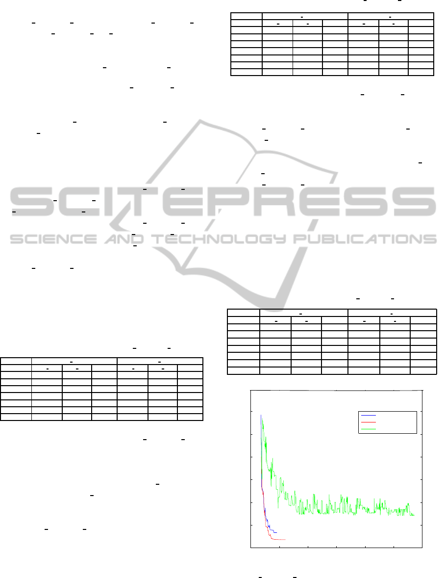
sity of the population after a few generations (Figure
2).
Table 4: Performances of AGAGD
Newman clus2.
Instance min weight min edge
best dev avg dev cpu(s) best dev avg dev cpu(s)
Celar06 0.38 11.18 17 0.35 11.86 17
Celar07 0.11 41.49 85 0.06 15.61 111
Celar08 1.52 11.83 290 6.87 29.38 197
Graph05 0.00 2,71 24 0.00 4.52 22
Graph06 0.07 15.74 200 0.00 11.83 172
Graph11 1.62 44.96 820 0.81 30.94 957
Graph13 13.67 50.92 2004 6.73 39.61 2171
6.4.2 Experiments on AGAGD Newman cut
Table 5 presents the results obtained with the
AGAGD Newman cut algorithm for both min weight
and min
edge variants. These results clearly
show a worse performance than the previous al-
gorithm both in terms of CPU time and best
dev
and avg dev. Indeed in this version, unlike the
AGAGD
Newman clus, the algorithm convergesvery
slowly (Figure 2). By performing the crossover on the
cuts, which are by definition less dense regions of the
problem, the cost of the solution tends to deteriorate
than to improve. When this degradation is significant,
the mutation operator struggles to repair it. Therefore,
the quality of the chromosomes tends to worsen over
the generations and the convergencethe algorithm be-
comes very slow.
Table 5: Results of AGAGD
Newman cut.
Instance min weight min edge
best dev avg dev cpu(s) best dev avg dev cpu(s)
Celar06 5.10 21.54 237 3.98 22.57 301
Celar07 50.15 426.71 812 41.66 469.29 1102
Celar08 30.53 50.01 1029 39.31 72.90 1079
Graph05 0.00 3.61 43 0.00 9.95 52
Graph06 0.02 10.57 443 0.04 27.04 337
Graph11 3.70 226.64 1807 46.20 335.55 1104
Graph13 16.22 118.82 5439 145.79 281.76 1724
0 200 400 600 800 1000 1200
3000
4000
5000
6000
7000
8000
9000
10000
AGAGD_clus
AGAGD_clus_cut
AGAGD_cut
#Gen
Cost
Figure 2: Graph11 instance: comparing
AGAGD
Newman y.
AGAGD-AnAdaptiveGeneticAlgorithmGuidedbyDecompositionforSolvingPCSPs
87

6.4.3 AGAGD Newman clus cut
Two dual methods were presented in the previous sec-
tions which both show their advantages and draw-
backs. To benefit from the two methods, an hybrid
heuristic called AGAGD
Newman clus cut is tested,
in which the crossover can either be performed on
the cluster or on the cut. Table 6 presents the
results of this heuristic both for min
weight and
min edge variants. The results obtained show that
this variant presents an important gain in terms of
CPU time as compared with those obtained by us-
ing AGA (Table2), especially for the min
edge vari-
ant. One can observe a significant improvement of
the results as compared with those obtained with the
two previous approaches. Notice that some perfor-
mances in terms of best
dev were reached, while
they were never obtained with AGA (Table 2) (see
Celar07 and Graph13). However, although the aver-
age performances avg
dev are improved as compared
with those obtained with AGAGD
Newman clus2
(Table 4) and AGAGD Newman cut (Table 5), they
still remain worse than those obtained with AGA
(Table 2). This is explained by the large num-
ber of variables involved in the crossover. This
means that AGAGD
Newman clus cut offers a good
compromise between AGAGD
Newman clus and
AGAGD Newman cut because the integration of
the two crossover operators Crossover clus and
Crossover
cut allows the algorithm to converge rela-
tively quickly, while maintaining some diversification
level. This avoids a premature convergence, thanks to
the Crossover
clus crossover (Figure 2) while a min-
imum diversification is maintained. This has enabled
to achieve almost near optimal results and even opti-
mal ones quickly.
Table 6: Performances of AGAGD
Newman clus cut.
Instance min weight min edge
best dev(%) avg dev cpu best dev avg dev cpu
Celar06 0.14 10.50 26 0.29 9.94 23
Celar07 0.08 25.18 193 0.00 10.73 149
Celar08 1.9 8.77 357 4.19 13.74 281
Graph05 0.00 1.80 31 0.00 2.26 26
Graph06 0.00 8.82 272 0.00 1.57 219
Graph11 1.36 49.64 1036 2.56 24.48 900
Graph13 4.61 41.63 2428 1.29 41.48 1556
6.5 AGA vs AGAGD
Table 6 summarizes some selected results obtained
by AGA and AGAGD algorithms. While we notice
the degradation of the parameter avg
dev in AGAGD,
let us note nonetheless improving some best
cost and
reduced time resolution especially on the most diffi-
cult instances.
Table 7: Comparing AGA and AGAGD.
Instance AGA AGAGD
best dev(%) avg dev cpu best dev avg dev cpu
Celar06 0.00 0.38 28 0.14 10.50 26
Celar07 0.02 0.05 212 0.00 10.73 149
Celar08 0.00 0.76 396 1.9 8.77 357
Graph05 0.00 0.00 27 0.00 1.80 31
Graph06 0.02 0.12 196 0.00 1.57 219
Graph11 1.26 3.60 1435 0.81 30.94 957
Graph13 3.77 6.94 2619 1.29 41.48 1556
7 CONCLUSION &
PERSPECTIVES
The aim of this work was to solve Partial Constraint
Satisfaction Problems close to the optimum in the
shortest time possible. To this aim, an Adaptive
Genetic Algorithm Guided by Decomposition called
AGAGD
x y was proposed. The name of the algo-
rithm is indexed by x and y, where x is for the generic
decomposition and y is for the generic genetic oper-
ator. In fact, the AGAGD
x y algorithm is doubly
generic because it fits several decomposition methods
and can accept several heuristics as crossover opera-
tor as well.
• For the decomposition step, two variants of
the well known decomposition algorithm due to
Newman were used, namely the min
edge and
min
weight variants.
• As crossover operators, three heuristics
called Crossover
clus, Crossover cut and
Crossover clus cut were proposed.
The first results obtained on MI-FAP problems are
promising. Indeed, the execution time was every-
where significantly reduced as compared with that ob-
tained with the previous AGA algorithm, while a de-
creasing of average quality of the solutions must be
accepted in some cases.
These early positive investigations encourage to fol-
low this direction of research and enhance the current
results. In the short term, it is planned to investigate
other heuristics in order to improve the crossover op-
erator. Moreover, a local repairing method can be as-
sociated with AGAGD
x y after each crossover step.
Last, it would be also interesting to deploy this ap-
proach on other multi-cut decomposition or tree de-
composition methods as well as on other PCSP appli-
cations.
REFERENCES
Aardal, K., Van Hoessel, S., Koster, A., Mannino, C., and
Sassano, A. (2007). Models and solution techniques
ICAART2015-InternationalConferenceonAgentsandArtificialIntelligence
88

for frequency assignment problems. Annals of Oper-
ations Research, 153:79–129.
Allouche, D., Givry, S., and Schiex, T. (2010). Towards
parallel non serial dynamic programming for solving
hard weighted csp. In Proceedings of CSP’ 2010,
pages 53–60.
Audhya, G. K., Sinha, K., Ghosh, S. C., and Sinha, B. P.
(2011). A survey on the channel assignment problem
in wireless networks. Wireless Communications and
Mobile Computing, 11(5):583–609.
CALMA-website (1995). Euclid Calma project.
ftp://ftp.win.tue.nl/pub/techreports/CALMA/.
Colombo, G. and Allen, S. M. (2007). Problem decomposi-
tion for minimum interference frequency assignment.
In Proceedings of the IEEE Congress on Evolutionary
Computation, Singapore.
Csardi, G. and Nepusz, T. (2006). The igraph software
package for complex network research. InterJournal,
Complex Systems, 1695(5).
Fontaine, M., Loudni, S., and Boizumault, P. (2013).
Exploiting tree decomposition for guiding neighbor-
hoods exploration for vns. RAIRO Operations Re-
search, 47(2):91–123.
Girvan, M. and Newman, M. (2002). Community struc-
ture in social and biological networks. Proceedings of
the National Academy of Sciences of the USA, pages
7821–7826.
Hale, W. K. (1980). Frequency assignment: Theory and
applications. Proceedings IEEE, 68(12):1497–1514.
Kolen, A. (2007). A genetic algorithm for the partial bi-
nary constraint satisfaction problem: an application
to a frequency assignment problem. Statistica Neer-
landica, 61(1):4–15.
Koster, A., Van Hoessel, S., and Kolen, A. (2002). Solv-
ing partial constraint satisfaction problems with tree
decomposition. Network Journal, 40(3):170–180.
Lee, L. H. and Fan, Y. (2002). An adaptive real-coded
genetic algorithm. Applied Artificial Intelligence,
16(6):457–486.
Loudni, S., Fontaine, M., and Boizumault, P. (2012). Ex-
ploiting separators for guiding vns. Electronic Notes
in Discrete Mathematics.
Maniezzo, V. and Carbonaro, A. (2000). An ants heuristic
for the frequency assignment problem. Computer and
Information Science, 16:259–288.
Metzger, B. H. (1970). Spectrum management technique.
38th National ORSA Meeting, Detroit.
Newman, M. (2004). Fast algorithm for detecting com-
munity structure in networks. Physical Review,
69(6):066133.
Ouali, A., Loudni, S., Loukil, L., Boizumault, P., and Leb-
bah, Y. (2014). Cooperative parallel decomposition
guided vns for solving weighted csp. pages 100–114.
Sadeg-Belkacem, L., Habbas, Z., Benbouzid-Sitayeb, F.,
and Singer, D. (2014). Decomposition techniques
for solving frequency assignment problems (fap) a
top-down approach. In International Conference on
Agents and Artificial Intelligence (ICAART 2014),
pages 477–484.
Schaeffer, S. E. (2007). Graph clustering. Computer Sci-
ence Review, 1:27–64.
Tate, D. M. and Smith, A. E. (1995). A genetic approach
to the quadratic assignment problem. Computers &
Operations Research, 22(1):73–83.
Voudouris, C. and Tsang, E. (1995). Partial constraint sat-
isfaction problems and guided local search. Technical
report, Department of Computer Science, University
of Essex. Technical Report CSM-25.
Zhou, Z., Li, C.-M., Huang, C., and Xu, R. (2014). An
exact algorithm with learning for the graph coloring
problem. Computers & Operations Research, 51:282–
301.
AGAGD-AnAdaptiveGeneticAlgorithmGuidedbyDecompositionforSolvingPCSPs
89