
Geometric Edge Description and Classification in Point Cloud Data with
Application to 3D Object Recognition
Troels Bo Jørgensen, Anders Glent Buch and Dirk Kraft
The Maersk Mc-Kinney Moller Institute, University of Southern Denmark, Campusvej 55, Odense, Denmark
Keywords:
Edge Detection, Object Recognition, Pose Estimation.
Abstract:
This paper addresses the detection of geometric edges on 3D shapes. We investigate the use of local point
cloud features and cast the edge detection problem as a learning problem. We show how supervised learning
techniques can be applied to an existing shape description in terms of local feature descriptors. We apply our
approach to several well-known shape descriptors. As an additional contribution, we develop a novel shape de-
scriptor, termed Equivalent Circumference Surface Angle Descriptor or ECSAD, which is particularly suitable
for capturing local surface properties near edges. Our proposed descriptor allows for both fast computation
and fast processing by having a low dimension, while still producing highly reliable edge detections. Lastly,
we use our features in a 3D object recognition application using a well-established benchmark. We show that
our edge features allow for significant speedups while achieving state of the art results.
1 INTRODUCTION
Edge detection in general is a highly investigated
topic in computer vision, mainly due to the possibil-
ity of condensing the input observations with a lim-
ited loss of information. This is beneficial also for 3D
applications, e.g., point cloud enrichment (Gumhold
et al., 2001) and pose estimation (Buch et al., 2013a),
since it can decrease computation times. For these
reasons, 3D edge detection should be fast, and it
should be easy to use for general point clouds, con-
taining noise and varying sampling densities. A 3D
edge detection example is shown in Figure 1.
Several other methods have been proposed to tack-
led the issue, including (Gumhold et al., 2001; Guy
and Medioni, 1997; Pauly et al., 2002; Pauly et al.,
2003). These methods tend to rely on complex hand-
crafted analyses of large local neighborhoods in order
to determine stable edge confidences. For this reasons
they become computationally expensive.
We propose to use a staged approach to produce a
simpler and faster algorithm, as done in 2D by e.g.,
Canny (Canny, 1986), but with very different pro-
cesses since we are dealing with 3D data. We first
estimate the edge direction using a local neighbor-
hood. Then we compute our local ECSAD descriptor
for describing the neighborhood, and then use the de-
scriptor to refine the edge direction estimate. Based
on this descriptor we provide two alternative methods
Figure 1: Left: a scene captured with a laser scanner (Mian
et al., 2006). Right: edge detector response using our
method (red means high confidence).
for finding an edge confidence: 1) directly using a cur-
vature estimate produced by our descriptor or 2) us-
ing machine learning techniques with labeled training
data. Finally, we adopt a non-maximum suppression
technique similar to that of Canny for our 3D edges
to arrive at a more condensed representation of point
clouds, which is desirable for matching tasks in e.g.,
object recognition applications.
We evaluate both our curvature based and learning
based edge detectors against several other methods on
point cloud data from multiple sensor modalities. For
these experiments, we have manually annotated both
training and test data, which provides a benchmark for
comparing 3D edge detectors, and allows for future
extensions. In a final application, we apply our edge
333
Jørgensen T., Buch A. and Kraft D..
Geometric Edge Description and Classification in Point Cloud Data with Application to 3D Object Recognition.
DOI: 10.5220/0005196703330340
In Proceedings of the 10th International Conference on Computer Vision Theory and Applications (VISAPP-2015), pages 333-340
ISBN: 978-989-758-089-5
Copyright
c
2015 SCITEPRESS (Science and Technology Publications, Lda.)

representation to a 3D object recognition and 6D pose
estimation system and show how to achieve both high
recognition rates and significant speedups during this
process.
This paper is structured as follows. We start by
relating our work to other methods for edge detection
in Section 2. Then we present our descriptor which is
used for reliable edge detection in Section 3. We then
show in Section 4 how any descriptor can be used for
learning an edge detector. In Section 5 we present
a simple edge thinning scheme for point clouds. In
Section 6 we provide extensive experiments of vari-
ous edge detectors, and we additionally show how to
use our features for 3D object recognition. Finally,
we make concluding remarks in Section 7.
2 RELATED WORK
The majority of edge detectors have been developed
for 2D images, and one of the most common edge de-
tection algorithms is the Canny edge detector (Canny,
1986), which revolves around semi-global methods in
order to capture more salient features. In (Choi et al.,
2013), Canny based methods were applied to RGB-D
images from a Kinect camera in order to determine
geometric and color based edges in organized point
clouds.
Geometric edge detection in general 3D data
structures has also gained some attention. For in-
stance, (B
¨
ahnisch et al., 2009; Monga et al., 1991)
have implemented edge detector in voxel based 3D
images. These methods are largely extensions of the
Canny detector to 3D, with a few modification to re-
duce computation times.
For unorganized point clouds, local point or direc-
tion information has been exploited to detect edges.
In (Guy and Medioni, 1997) a PCA analysis of the
normals is made in order to determine how much the
surface varies. The work in (Pauly et al., 2003) pro-
poses to use the curvature estimates at several differ-
ent scales in order to determine a edge confidence.
Gumhold et al. (Gumhold et al., 2001) propose to use
a more complex combination of eigenvalues, eigen-
vectors and other curvature estimates in order to de-
termine a handcrafted edge confidence. This paper
also proposes to use a minimum spanning tree where
short branches are removed in order to do edge thin-
ning. A final spline fitting provides a smoother visual
representation.
In this work, we address the detection of 3D edges
in unorganized (or unstructured) point clouds. Such
edges often occur at orientation discontinuities where
two planar surfaces coincide. For this task, we have
derived an appropriate local shape descriptor, termed
ECSAD, which can be used for detecting edges, either
directly by a curvature estimate produced by the de-
scriptor or by learning an edge classifier in descriptor
space. To our knowledge, current shape descriptors,
such as e.g., (Johnson and Hebert, 1999; Mian et al.,
2006; Rusu et al., 2009; Tombari et al., 2010), are
focused strictly on the task of describing local shape
patches of arbitrary geometry for use at a later match-
ing stage.
Finally, we motivate the use of our edges and asso-
ciated descriptors in a 3D object recognition applica-
tion, where we also apply our descriptor for matching,
leading to state of the art recognition performance.
We note that, similar to our work, the edges detected
in (Buch et al., 2013a; Choi et al., 2013) were also
applied for object registration, in the latter case based
on point pair features, originally proposed by (Drost
et al., 2010). However, the edge detection method
of (Choi et al., 2013) is restricted to organized RGB-
D images, and not general 3D shapes, which renders
evaluations against our work impossible. We do, how-
ever, compare ourselves with the registration algo-
rithm of (Drost et al., 2010).
3 LOCAL SURFACE
DESCRIPTOR FOR EDGE
DETECTION
We have developed a local descriptor focusing on
edge detection and classification, partly to determine
the direction of the edges, and partly to be used in su-
pervised learning for edge detection. The descriptor
is a vector of relative angles between opposing sides
of the edge, which we have found to provide a good
description for geometric edges caused by orientation
discontinuities. Before descriptor estimation, the in-
put point cloud is down-sampled to a uniform resolu-
tion. The radius of the spherical support (the area that
influences the descriptor) is a free parameter, but we
have consistently used a value of five times the down-
sampling resolution for simplicity.
As will be explained in the following, our descrip-
tor uses a spatial decomposition which gives each spa-
tial bin approximately the same circumference. Con-
trary to other descriptors that use histograms, our uses
simple but stable angle measurements. For these rea-
sons, we term our descriptor Equivalent Circumfer-
ence Surface Angle Descriptors (ECSAD).
Spatial Decomposition. Similar to other local sur-
face descriptors, we use a spatial decomposition,
which is illustrated in Figure 2 by a cross section
VISAPP2015-InternationalConferenceonComputerVisionTheoryandApplications
334

Figure 2: Left: visualization of the computed descriptor at
an edge point with a tangent direction (red) and a surface
normal (blue), please see text for a description how these
are defined. The spatial bins are intersected by a number of
surface points, and the contents of each bin is visualized by
the plane patch spanned by these intersecting surface points.
Right: a cross section showing the tangent plane of the local
support, showing the decomposition used by our descriptor.
through the spherical region. Our descriptor splits the
local space along the radial and azimuth dimensions,
but not along the elevation as in e.g., (Frome et al.,
2004; Tombari et al., 2010). This choice is justified
by the fact that it is extremely rare that more than one
surface passes through the same azimuth bin at dif-
ferent elevations, thus resulting in a high fraction of
empty bins along the elevation. This again leads to in-
stabilities towards position noise, and we have found
this to produce worse results for edge detection and
description. In Figure 2, left this can be seen as noise
in the elevation of the surface patches.
Instead, we have devised a more sophisticated and
uneven binning of the azimuth dimension (see Fig-
ure 2, right). We start by splitting the local space into
six equiangular azimuth bins of 60
◦
through all radial
levels (bold lines). Now, for each of these six azimuth
bins, we increase the number of azimuth splittings by
one for each radial increment, giving a total increase
of six azimuth bins per radial level (thin lines). This
leads to an almost uniform angular coverage of all the
bins in the azimuth dimension, and we have found this
to produce much better performance than simply us-
ing an equal number of azimuth bins at all radial lev-
els. We have tested different numbers of radial lev-
els and found a good compromise between specificity
and robustness for four radial levels (note that only
three radial levels are shown in Figure 2, right).
Reference Frame Estimation and Bin Angles.
The first step of the algorithm is to estimate the sur-
face normal and a tangential edge direction of the
center point which is to be described. This is done
by the eigendecomposition of the scatter matrix of
all the points in the support, giving the direction and
normal along the eigenvectors corresponding to the
largest and smallest eigenvalues, respectively. The lo-
cal reference frame (LRF) x- and z-axis is given by
these two vectors, and the y-axis by their cross prod-
uct. Then we map each of the supporting points into
the correct spatial bin based on its radial and azimuth
coordinates relative to the center point. This is done
using the direction vector from the center point to the
supporting point. The radial component is immedi-
ately given by the norm of this vector, while the az-
imuth component is given by the relative angle be-
tween this vector and the x-axis, measured in the tan-
gent plane of the normal vector. For each bin, we
now compute the relative angle between the surface
normal and the direction vector to each point in the
spatial bin. This angle is then averaged over all points
that fall in the same spatial bin, giving a single an-
gle measurement per spatial bin. After the angles to
the individual bins have been determined, an interpo-
lation strategy is used to assign values to bins with
missing information, i.e., bins which have no points.
The interpolation value of a bin is performed by
averaging the angles of up to five neighbor bins: one
at a lower radial level, two next to the bin at the same
radial level, and the two closest at a higher radial
level. The neighbors at the same and at the higher
radial level are only used if they contain points and
thereby an angle measurement. The interpolation then
starts from the center and moves outwards. At the first
radial level, the bin angle at a lower radial level de-
fined as zero. This ensures a value will be assigned to
every bin.
Description Using Sum of Angles. At an edge
point, the x-axis separates two surfaces meeting at the
center point. Our descriptor tries to approximate the
angle between these two surfaces using the individual
angle measurements of the spatial bins. To achieve
this we identify opposing spatial bins, i.e., bins that
have the same radial component but separated by an
azimuth angle of π. We now take the sum of angles of
each opposing bin pair, reducing the number of angle
observations by a factor of two (green lines in Fig-
ure 2, right). Each angle sum approximates the angle
between the coinciding surfaces, but this summation
also makes our descriptor invariant to the sign of the
x-axis, which is desirable, since this direction is am-
biguous.
Reference Frame Refinement and Curvature Es-
timate. A special case occurs in concave regions,
i.e., at points where the normal vector (z-axis) has
an angle of less than π/2 to the two opposing sur-
faces. This can easily be measured by checking if the
average of the sum of angles defined above is larger
than π. In such cases, we negate the y- and z-axis
of the LRF. Finally, we perform a refinement of the
x-axis by treating the sum of angle entries as a local
2D map, where each entry equals the angle measure-
ment weighted by the radial component. We compute
GeometricEdgeDescriptionandClassificationinPointCloudDatawithApplicationto3DObjectRecognition
335

the eigendecomposition of the covariance matrix of
this local 2D map of weighted angle entries, and the
edge direction will now be better approximated by the
in-plane eigenvector of the smallest eigenvalue. We
rotate the LRF around the z-axis to coincide with the
updated x-axis. Using this refined RF, we now recom-
pute all the sum of angle measurements to get a more
robust descriptor.
As a side effect, the biggest eigenvalue of the lo-
cal 2D map computed above provides a good esti-
mate of the the local curvature around the edge. In
Section 6 we show results of using this measure for
edge detection. In all the experiments, we have used
four radial levels, leading to a descriptor dimension of
(6 +12 + 18 + 24)/2 = 30
In order to use the descriptor in pose estimation,
it is beneficial to orient the normals to point outwards
from the underlying objects. This is done to improve
correct match rates, since it enables distinction be-
tween convex and concave regions. For scenes, this
is done by rotating the scene normals towards a view-
point. For models it is done based on a technique pro-
posed by (Hoppe et al., 1992).
If the normal signs are changed, the descriptors
are updated, similarly to how concave regions are ori-
ented to produce similar descriptors for concave and
convex regions to simplified edge detection.
4 SUPERVISED LEARNING FOR
EDGE DETECTION
Using our ECSAD descriptors, a random forest (RF)
classifier (Breiman, 2001) was trained in order to de-
termine edge confidences in point clouds containing
structured noise, such as point clouds captured by
range sensors.
The training dataset consists of manually labeled
point clouds, captured by Kinect cameras, stereo cam-
eras and sampled from CAD models. Examples of
labeled point clouds from these different sources are
seen in Figure 3. Here the red lines are positive edge
examples, the blue lines are ignored due to uncer-
tainty of the human annotator, and the rest of the
points are negative examples. We trained using four
CAD models, two stereo scenes, two Kinect scenes
and three Kinect views of different objects. All in all
this provided more than 12500 positive and 285000
negative training examples.
These data, along with the local feature descrip-
tors computed over the full point clouds, were then
used in order to train the random forests. Based on
multiple runs over different parameters, we found that
a point cloud resolution of 4 mm, a support radius of
Figure 3: Examples of labeled point clouds from various
sources used for training (relative sizes are not preserved
in this figure). Ground truth edges (red) are used as pos-
itive examples, and transition regions between edges and
non-edges (blue) are discarded during training. The rest of
the points are non-edges, which are used as negative exam-
ples. Left: an ideal CAD model, resampled to a point cloud.
Middle: a real scene with projected texture pattern, recon-
structed by a block matching algorithm. Right: a partial
view of a textured object, taken from the RGB-D Dataset
(Lai et al., 2011).
20 mm, and an RF with 30 trees and a maximum tree
depth of 15 provided good results. Similar figures
hold for the other methods which we will compare
against in Section 6.
In the test phase, a new point cloud with computed
feature descriptors is fed to the RF classifier. The out-
put edge confidence at a feature point is then simply
given by the number of trees in the RF that classify
the feature as an edge.
A smoothness technique is applied to the edge
confidences, which is beneficial as an extra step be-
fore applying non-maximum edge suppression for
thinning the edge map. This is simply implemented
by determining the ten closest points to the edge point
in question and averaging the edge confidences. After
this step, the cloud is ready for non-maximum edge
suppression.
5 EDGE THINNING
For some applications, e.g., object recognition, a
sparse representation can be desirable. One of the
simplest solutions in our case is to use a non-
maximum edge suppression technique. This is im-
plemented by determining the 20 closest edge points
to a potential edge. Denote the current center point as
p
C
and a neighbor as p
N
, both with associated edge
directions d
C
and d
N
and edge confidences c(p
C
) and
c(p
N
). To determine whether p
C
suppresses p
N
, three
criteria are used. First, p
C
must have the highest edge
confidence:
c(p
C
) > c(p
N
) (1)
Secondly, we impose the following collinearity con-
straint:
∠ (d
C
, p
N
− p
C
) >
3
8
· π (2)
VISAPP2015-InternationalConferenceonComputerVisionTheoryandApplications
336

Figure 4: Left: a table scene from the RGB-D Dataset. Mid-
dle: edge detector responses. Right: remaining edges after
non-maximum suppression.
Figure 5: Edge responses after non-maximum suppression.
Left: A real scene with projected texture pattern, recon-
structed by a block matching algorithm. Right: An ideal
CAD model resampled to a point cloud.
This ensures that points on the same line do not sup-
press each other. Thirdly, we require the following:
∠ (d
C
,d
N
) <
π
4
(3)
This ensures that orthogonal edges do not suppress
each other. As an optimization, we check (1)–(3)
bidirectionally, i.e., if a neighbor point suppresses the
center point, the center point is discarded. This step is
done to reduce the number of neighborhood searches,
which is computationally expensive in point clouds.
A visualization of this suppression process is
shown for a Kinect scene in Figure 4. We note that
the thinning is an optional step, and in this paper we
use it only in the final object recognition application.
For a fair comparison of edge detectors, it is more ap-
propriate to directly use the output edge confidences,
as we will show in Section 6.1.
Figure 1 and Figure 5 show the edge response af-
ter line thinning for three other point clouds . Here it
is seen that the detector has a decent response for all
data sources, but it should be noted that the response
near borders is poor, partly due to higher noise lev-
els in these areas. In the Kinect point cloud it is also
seen that the responses become poor at the most dis-
tant parts of the scene, where the noise and quantiza-
tion levels are particularly high.
6 EXPERIMENTS
In this section we provide experimental results both
for our edge detection algorithms, and for an object
recognition application. All algorithms were imple-
mented in single-threaded C++ applications, primar-
ily using functionality from the Point Cloud Library
1
(Rusu and Cousins, 2011). OpenCV
2
was used for its
interface to machine learning algorithms.
The algorithms was evaluated using an Intel core
i3 3217U, 1.8GHz with 4GB RAM. This computer
is roughly equivalent to the one used by Drost et al.
(Drost et al., 2010).
We have tested a range of parameters for our
method, and the performance varies between different
data sources (Kinect, CAD and stereo). A full evalua-
tion of these parameters and their influence on the per-
formance on various data sources is beyond the scope
of this paper. In this section we present results using
the previously mentioned parameter values, providing
good results in general for all data sources.
6.1 Quantitative Evaluation of Edge
Detectors
For the purpose of evaluating the strength of our edge
detector, we have created test data in a similar man-
ner to the training data (see Figure 3). The test set
was generated using two CAD models, two stereo
scenes and two Kinect scenes, providing more than
6000 positive and 170000 negative test examples, re-
spectively. We split the test set into three different
categories (CAD, stereo and Kinect), as we have ob-
served quite a varying performance across the differ-
ent data sources. Note that the training set has not
been split; only one training pass over the full train-
ing set is performed. All training and test data are
publicly available on our web site.
3
We train an RF classifier using our ECSAD de-
scriptor. Additionally, we perform the same proce-
dure using two recent shape descriptors, the Signature
Histogram of Orientations (SHOT) (Tombari et al.,
2010) and the Fast Point Feature Histogram (FPFH)
(Rusu et al., 2009). Both features have been widely
used for surface description.
In addition to the RF test, we evaluate the use
of the internal curvature estimate produced by our
descriptor for directly providing an edge confidence.
For comparison, we also include in our test other cur-
vature estimates, namely the total surface variation
(Pauly et al., 2002) (termed Curvature) and a multi-
scale extension of this algorithm (Pauly et al., 2003)
(termed ScaleCurv). In these two algorithms, the cur-
vature is estimated using the three eigenvalues of the
scatter matrix of the supporting points around a point,
1
http://pointclouds.org
2
http://opencv.org
3
https://sites.google.com/site/andersgb1/projects/3d-edge-
detection
GeometricEdgeDescriptionandClassificationinPointCloudDatawithApplicationto3DObjectRecognition
337
0 0.1 0.2 0.3 0.4 0.5 0.6 0.7 0.8 0.9 1
0
0.1
0.2
0.3
0.4
0.5
0.6
0.7
0.8
0.9
1
1-precision
recall
CAD
0 0.1 0.2 0.3 0.4 0.5 0.6 0.7 0.8 0.9 1
0
0.1
0.2
0.3
0.4
0.5
0.6
0.7
0.8
0.9
1
1-precision
recall
Stereo
0 0.1 0.2 0.3 0.4 0.5 0.6 0.7 0.8 0.9 1
0
0.1
0.2
0.3
0.4
0.5
0.6
0.7
0.8
0.9
1
1-precision
recall
Kinect
ECSAD_RF
SHOT_RF
FPFH_RF
ECSAD_Curv
Curvature
ScaleCurv
ECSAD RF SHOT RF FPFH RF ECSAD Curv Curvature ScaleCurv
9.23 s 18.17 s 16.0 s 7.66 s 9.02 s 18.8 s
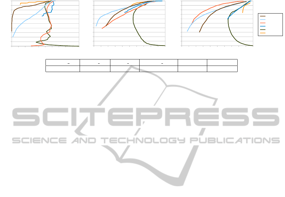
Figure 6: Performance curves in terms of (1 - precision) vs. recall for the CAD (left), stereo (middle) and Kinect (right) test
scenes. The bottom table shows the accumulated detection time for all six point clouds (in total ca. 176000 points) in the test
dataset. For the learned detectors, this includes both descriptor computation and RF classification.
simply by dividing the smallest eigenvalue by the sum
of all three eigenvalues.
In Figure 6 we show results for all three data
sources as (1 - precision) vs. recall curves, which is a
standardized way to evaluate interest point detectors
(Mikolajczyk and Schmid, 2005). For the ideal CAD
models, which have noise-free edges, we observe a
very high performance of the multi-scale curvature as
edge confidence. Our learned detector comes close in
performance, and shows a very high initial precision
at low recall. For the real stereo and Kinect data, the
performance of the curvature based detectors imme-
diately drops, and the learned detectors become su-
perior. For the Kinect data with the highest noise,
the FPFH detector shows the best performance. Our
learned detector shows comparable performance for
all three data sources. In addition to this, our descrip-
tor is computationally efficient–almost twice as fast
as SHOT and FPFH. In addition, the SHOT descrip-
tor has a dimension more than ten times higher than
both FPFH and ECSAD.
6.2 Application: 3D Object Recognition
In order to assess the benefits of edge detection for
another application, we applied a previously proposed
point cloud registration algorithm to our features. The
method is presented in (Buch et al., 2013b) and is
based on RANSAC (Fischler and Bolles, 1981), with
a crucial optimization step used for early rejection of
point samples that are unlikely to produce valid pose
hypotheses. We further improve the method by allow-
ing for multiple feature matches within a predefined
radius in descriptor space. The algorithm is presented
below.
Initialization:
1. The object and scene surfaces are down-sampled
to a voxel size of 3 mm to ensure a uniform point
cloud resolution.
2. Edges are detected within both the object and
scene point clouds using the learned RF detector,
using ECSAD descriptors computed with a sup-
port radius of 15 mm. Non-maximum suppression
is applied to reduce the number of features. The
descriptors are stored for use below.
3. For each object edge feature, we use k-d trees
to search for all matching feature descriptors in
the scene within a radius of one unit in descriptor
space.
Iterate:
1. Three random feature points are sampled on the
object. For each of these points a random scene
correspondence is retrieved from the list of corre-
spondences generated in step 3 of the initializa-
tion.
2. Apply the pre-rejection of (Buch et al., 2013b):
if any of the distances between the three object
points differs more than 10 % from the equivalent
distance between the corresponding scene points,
continue to the next iteration.
3. A pose hypothesis is generated based on the three
matches.
4. The pose is applied to the object point cloud,
and we count the number of inliers supporting
the pose by an Euclidean proximity threshold of
3 mm. Additionally, we require that the aligned
normal vectors have a relative angle less than π/3.
If the number of inliers satisfying both these con-
ditions is higher than 15 % of the number of ob-
ject points, we break out and consider the object
as recognized.
The pre-rejection step makes the search for valid
poses very fast, so we run the algorithm for a max-
VISAPP2015-InternationalConferenceonComputerVisionTheoryandApplications
338

imum of 100000 iterations. In case all 100000 itera-
tions are completed without finding a pose with more
than 15 % inliers, the best pose is chosen to ensure
recognition of highly occluded objects. Finally the
determined pose is refined by ten iterations of the iter-
ative closest point algorithm (Besl and McKay, 1992).
As an additional test, we also implemented our
method with the full set of ECSAD features at all
down-sampled surface points, not only at the edge
features. We have tested our algorithms on the well-
known laser scanner dataset by Mian et al. (Mian
et al., 2006), consisting of four complete objects to be
recognized in view-based 50 test scenes.
4
For com-
parison, we present previous results for three state
of the art methods: Spin images by Johnson and
Hebert (Johnson and Hebert, 1999), Tensor matching
by Mian et al. (Mian et al., 2006), and finally the
PPF registration by Drost et al. (Drost et al., 2010).
The results are presented as occlusion vs. recognition
rate, similarly to how (Mian et al., 2006) evaluated the
original algorithms on the dataset. Occlusion is the
percentage of the object which is visible, and recog-
nition rate is the relative number of times an object
is recognized in the 50 scenes. An object pose is ac-
cepted if it diverges with less than 12
◦
and 5 mm from
the ground truth pose, which is similar to the criterion
used in (Drost et al., 2010).
For our surface-based method, we see a high per-
formance, which indicates a high performance of
the registration algorithm. The edge features, be-
ing more discriminative, show an even higher per-
formance, giving the best recognition results at the
highest occlusion rates. Additionally, we report the
average recognition time per object, which for our al-
gorithm includes both ECSAD computation, edge de-
tection by the classifier and non-maximum suppres-
sion. These numbers clearly show the gain of using
our sparse edge representation, giving a significant
speedup relative to both the surface-based registration
algorithm and the fast PPF registration.
7 CONCLUSION AND FUTURE
WORK
A new edge detection approach for 3D point clouds
from various sources has been developed, focusing
on speed and overall performance. In these aspects
our detector shows superior performance compared to
other methods, even with limited parameter tuning.
A RANSAC based pose estimation algorithm was
developed, which shows that using edges can signif-
4
http://www.csse.uwa.edu.au/∼ajmal/recognition.html
60 65 70 75 80 85 90 95
0
0.1
0.2
0.3
0.4
0.5
0.6
0.7
0.8
0.9
1
ECSAD (edges) – 0.731 s
ECSAD (surfaces) – 3.21 s
PPF (slow) – 85.0 s
PPF (fast) – 1.97 s
Tensor matching – 90.0 s
Spin images – 2 hours
Occlussion %
Recognition rate
Figure 7: Comparison of our surface- and edge-based
recognition systems with other works. The upper figure
shows different pose estimation algorithm performances in
terms of recognition-occlusion curves along with average
running times per object. The bottom figure shows the first
scene of the dataset, also shown in Figure 1. The magenta
objects are the determined poses, so in this scene all objects
have been correctly recognized.
icantly improve the runtime of 3D recognition algo-
rithms. Furthermore the simple pose estimation ap-
plication matches the performance of state of the art
recognition systems on an established laser scanner
benchmark, while being significantly faster.
In future work, a robustness study of the local ref-
erence frame compared with other reference frame
estimation algorithms would be highly interesting.
Since the descriptor has the best performance for a
relatively small support radius, it would be interesting
to apply the edges in higher level descriptors to deter-
mine if such an approach can result in a higher match
rate for large noisy scenes. It would also be interest-
ing to investigate the performance of the descriptor
if it was used in a Hough-like voting algorithm in-
stead of a RANSAC based approach. It is doubtful
that this will increase the speed for the tested recogni-
tion dataset, but it may improve the recognition rate in
more complex scenarios, where segmentation is often
performed. In this context it would also be interesting
to investigate if the edges can be used in a point cloud
segmentation algorithm.
GeometricEdgeDescriptionandClassificationinPointCloudDatawithApplicationto3DObjectRecognition
339

ACKNOWLEDGEMENTS
The research leading to these results has received
funding by The Danish Council for Strategic Re-
search through the project Carmen and from the Euro-
pean Community’s Seventh Framework Programme
FP7/2007-2013 (Specific Programme Cooperation,
Theme 3, Information and Communication Technolo-
gies) under grant agreement no. 270273, Xperience.
REFERENCES
B
¨
ahnisch, C., Stelldinger, P., and K
¨
othe, U. (2009). Fast and
accurate 3D edge detection for surface reconstruction.
In Pattern Recognition, pages 111–120. Springer.
Besl, P. and McKay, N. D. (1992). A method for regis-
tration of 3-d shapes. Pattern Analysis and Machine
Intelligence, IEEE Transactions on, 14(2):239–256.
Breiman, L. (2001). Random forests. Machine learning,
45(1):5–32.
Buch, A. G., Jessen, J. B., Kraft, D., Savarimuthu, T. R.,
and Kr
¨
uger, N. (2013a). Extended 3D line segments
from RGB-D data for pose estimation. In Scandina-
vian Conference on Image Analysis (SCIA), pages 54–
65. Springer.
Buch, A. G., Kraft, D., Kamarainen, J.-K., Petersen, H. G.,
and Kruger, N. (2013b). Pose estimation using local
structure-specific shape and appearance context. In
Robotics and Automation (ICRA), 2013 IEEE Inter-
national Conference on, pages 2080–2087.
Canny, J. (1986). A computational approach to edge detec-
tion. Pattern Analysis and Machine Intelligence, IEEE
Transactions on, PAMI-8(6):679–698.
Choi, C., Trevor, A. J., and Christensen, H. I. (2013). RGB-
D edge detection and edge-based registration. In In-
telligent Robots and Systems (IROS), 2013 IEEE/RSJ
International Conference on, pages 1568–1575.
Drost, B., Ulrich, M., Navab, N., and Ilic, S. (2010). Model
globally, match locally: Efficient and robust 3D object
recognition. In Computer Vision and Pattern Recogni-
tion (CVPR), 2010 IEEE Conference on, pages 998–
1005.
Fischler, M. A. and Bolles, R. C. (1981). Random sample
consensus: a paradigm for model fitting with appli-
cations to image analysis and automated cartography.
Communications of the ACM, 24(6):381–395.
Frome, A., Huber, D., Kolluri, R., B
¨
ulow, T., and Malik, J.
(2004). Recognizing objects in range data using re-
gional point descriptors. In Proceedings of the Euro-
pean Conference on Computer Vision (ECCV), pages
224–237.
Gumhold, S., Wang, X., and MacLeod, R. (2001). Feature
extraction from point clouds. In Proceedings of 10th
international meshing roundtable, pages 293–305.
Guy, G. and Medioni, G. (1997). Inference of surfaces, 3D
curves, and junctions from sparse, noisy, 3D data. Pat-
tern Analysis and Machine Intelligence, IEEE Trans-
actions on, 19(11):1265–1277.
Hoppe, H., DeRose, T., Duchamp, T., McDonald, J., and
Stuetzle, W. (1992). Surface reconstruction from un-
organized points. In ACM SIGGRAPH Proceedings,
pages 71–78.
Johnson, A. E. and Hebert, M. (1999). Using spin im-
ages for efficient object recognition in cluttered 3D
scenes. Pattern Analysis and Machine Intelligence,
IEEE Transactions on, 21(5):433–449.
Lai, K., Bo, L., Ren, X., and Fox, D. (2011). A large-
scale hierarchical multi-view RGB-D object dataset.
In Robotics and Automation (ICRA), 2011 IEEE In-
ternational Conference on, pages 1817–1824.
Mian, A. S., Bennamoun, M., and Owens, R. (2006).
Three-dimensional model-based object recognition
and segmentation in cluttered scenes. Pattern Anal-
ysis and Machine Intelligence, IEEE Transactions on,
28(10):1584–1601.
Mikolajczyk, K. and Schmid, C. (2005). A perfor-
mance evaluation of local descriptors. Pattern Analy-
sis and Machine Intelligence, IEEE Transactions on,
27(10):1615–1630.
Monga, O., Deriche, R., and Rocchisani, J.-M. (1991). 3D
edge detection using recursive filtering: application
to scanner images. CVGIP: Image Understanding,
53(1):76–87.
Pauly, M., Gross, M., and Kobbelt, L. P. (2002). Efficient
simplification of point-sampled surfaces. In IEEE
Conference on Visualization, pages 163–170.
Pauly, M., Keiser, R., and Gross, M. (2003). Multi-scale
feature extraction on point-sampled surfaces. Com-
puter Graphics Forum, 22(3):281–289.
Rusu, R. B., Blodow, N., and Beetz, M. (2009). Fast point
feature histograms (FPFH) for 3D registration. In
Robotics and Automation, 2009. ICRA’09. IEEE In-
ternational Conference on, pages 3212–3217.
Rusu, R. B. and Cousins, S. (2011). 3D is here: Point cloud
library (PCL). In Robotics and Automation (ICRA),
2011 IEEE International Conference on, pages 1–4.
Tombari, F., Salti, S., and Di Stefano, L. (2010). Unique
signatures of histograms for local surface description.
In European Conference on Computer Vision (ECCV),
pages 356–369.
VISAPP2015-InternationalConferenceonComputerVisionTheoryandApplications
340
