
Impact on Bayesian Networks Classifiers
When Learning from Imbalanced Datasets
M. Julia Flores and Jos´e A. G´amez
Computing Systems Department – SIMD group (I3A), University of Castilla - La Mancha, Campus, 02071, Albacete, Spain
Keywords:
Bayesian Networks, Supervised Classification, Data Mining, Imbalanced Datasets, Naive Bayes.
Abstract:
In this paper we present a study on the behaviour of some representative Bayesian Networks Classifiers
(BNCs), when the dataset they are learned from presents imbalanced data, that is, there are far fewer cases
labelled with a particular class value than with the other ones (assuming binary classification problems). This
is a typical source of trouble in some datasets, and the development of more robust techniques is currently
very important. In this study, we have selected a benchmark of 129 imbalanced datasets, and performed an
analytical approach focusing on BNCs. Our results show good performance of these classifiers, that outper-
form decision trees (C4.5). Finally, an algorithm to improve the performance of any BNC is also given. We
have carried out an experimentation where we show how the using of oversampling of the minority class to
achieve the desired value for the imbalance ratio (IR), which is the division of the number of cases for the
majority class by the cases of the minority class. From this work we can conclude that BNCs show a very
good performance for imbalanced datasets, and that our proposal enhance their results for those datasets that
provided poor results.
1 INTRODUCTION
Supervised learning construct models from externally
supplied instances to produce general hypotheses,
which then make predictions about future instances.
In other words, the goal of supervised learning is to
build a concise function of the distribution of class la-
bels in terms of predictive attributes features. There
exist many families for these models, known as clas-
sifiers, for example decision trees, support vector ma-
chines, artificial neuralnetworks or rule systems. Any
kind of classifier is always used to assign class la-
bels to a set of testing instances where the values of
the predictor features are known, but the value of the
class label is unknown. In fact, a classifier is needed
to provide the correct class label for future or unseen
cases, for example determining if a manufacture piece
is defective based on a set of features extracted from
visual information (an image taken by a camera), or
determine if an e-mail is spam or not based on those
attributes that can be extracted from the correspond-
ing information (subject, sender, etc...).
Most classifier learning algorithms assume a rela-
tively balanceddistribution (Breiman, 1998), so when
there is an under-represented class, this poses a seri-
ous problem for them, and they generally have poor
generalisation performance on the minority class. In
real applications, the imbalance class scenery appears
more frequently than expected. For example, in med-
ical diagnosis the disease cases are usually quite rare
in global populations (where most of the people do
not suffer from the related disease). However, the
key task here is to detect which people have this dis-
ease. In this case, a classifier that provides a higher
identification rate on the disease category would pro-
vide better performance. Other fields of application
where imbalanced data naturally arise are fraud de-
tection, monitoring, text categorization, risk manage-
ment, etc... It happens in so many real problems that
it can be considered one of the top problems in data
mining today (Lopez et al., 2013).
Bayesian Network classifiers (BNCs) are
Bayesian Network (BN) models (Korb and Nichol-
son, 2010) specifically tailored for classification
tasks. There is a wide range of existing models that
vary in complexity and efficiency. All of them have in
common the ability to deal with uncertainty in a very
natural way, at the same time providing a descriptive
environment. In this work, we will focus on the
family of semi-naive (Kononenko, 1991) Bayesian
classifiers (Naive Bayes, AODE, TAN, kDB, etc.).
The capability of a BN to express relationships,
dependencies and independences between variables
(features in this case) is given by its associated graph
382
Flores M. and Gámez J..
Impact on Bayesian Networks Classifiers When Learning from Imbalanced Datasets.
DOI: 10.5220/0005201103820389
In Proceedings of the International Conference on Agents and Artificial Intelligence (ICAART-2015), pages 382-389
ISBN: 978-989-758-074-1
Copyright
c
2015 SCITEPRESS (Science and Technology Publications, Lda.)

(qualitative part), and these relationships are also
modelled with a second element, quantitative, that
forms a BN: probability distributions. In our opinion,
there are two main characteristics that have made
BNCs so popular: they provide predictions in terms
of probabilities (that could be interpreted as weights)
and they are easily and intuitively interpreted by non-
experts (thanks to the underlying graph). Empirically,
BNCs have also been successfully in many applica-
tion areas (Flores et al., 2012) such as Computing,
Robotics, Medicine, Healthcare, Finance, Banking
and Environmental Science.
This paper is organized as follows. In Section 2,
we review some previous work related to the current
one, and discuss the novelty of our approach. In Sec-
tion 3, we present the first part of our experiments,
where we analyse the behaviour of some BNCs in a
benchmarkof imbalanceddatasets. Section 4 presents
the final experimentation of the paper, from which
we conclude which is the algorithm to apply. Some
conclusions from these results are also given. Finally,
Section 5 provides a general discussion and future re-
search lines.
2 RELATED WORK
In (Lopez et al., 2013), authors present a very interest-
ing study where they identify which are the intrinsic
characteristics that affect when applying supervised
classification models on imbalanced datasets. In this
work authors pre-select a set of 66 datasets (subset
of those in Table 1). This work proves that Imbal-
ance Ratio (IR) is, of course, a very important factor
when working with imbalanced datasets, however,the
performance of classifiers can not be obtained for a
simple (linear) function with respect to this measure.
They see how other aspects can also influence, such
as the presence of small disjoints, the lack of density
in the training data, the overlapping between classes,
the identification of noisy data, the significance of the
borderline instances, and the dataset shift between the
training and the test distributions. The problem with
these other measures is that obtaining them is not an
easy task, and when it can be done with approximate
values, they suppose a high computing cost. Besides,
these depend on the particular problem to solve, while
we are interested in developing generaltechniques ap-
plicable to any dataset. That is why, we will firstly
work on the behaviour with respect to the IR value, in
combination with other graphical tools and plots.
The novelty of the current work is that it is
uniquely focused on the behaviour on BNCs, since
most of the works related to imbalanced datasets are
devoted to other kind of models, for example (Lopez
et al., 2013) uses Decision trees (C4.5), Support vec-
tor machines (SVMs) and the k-Nearest Neighbours
(kNN) model, which goes into the family of Instance
based learning. On the other hand, (Sun et al., 2007)
applies two kinds of systems: again C4.5 decision
tree and an associative classification system called
HPWR (H
igh-order Pattern and Weight-of- evidence
R
ule based classifier). We considered that there is an
open research line in the study of the behaviour of
BNCs with imbalanced data and performing a study
of how to approach this problem is the main aim of
this paper.
Another related work, where BNCs are used is
(Wasikowski and wen Chen, 2010), but this is not ap-
plicable to the available datasets, since the number of
attributes in our problems are too low, and the num-
ber of instances is comparatively few, so it does not
have sense to apply feature subset selection. In the
referred work they use datasets which are not origi-
nally imbalanced, and we wanted to apply BNCs to
real imbalanced datasets.
3 ANALYTICAL EXPERIMENTS
Here we will show the basis for our study and an ini-
tial experimental set-up, analysing their results.
3.1 Selected BNCs
The classification task consists of assigning one cate-
gory c
i
or value of the class variable C = {c
1
,...,c
k
}
to a new object ~e, which is defined by the assign-
ment of a set of values, ~e = {a
1
,a
2
,··· ,a
n
}, to the
attributes A
1
,...,A
n
. In the probabilistic case, this
task can be accomplished in an exact way by the ap-
plication of the Bayes theorem (Equation 1). How-
ever, since working with joint probability distribu-
tions is usually unmanageable, simpler models based
on factorizations are normally used for this problem.
In this work we apply four computationally efficient
paradigmsNaive Bayes (NB), KDB,TAN and AODE.
Our experimentswill also show that imbalanced prob-
lems does not benefit from more complex BNCs.
p(c|~e) =
p(c)p(~e|c)
p(~e)
. (1)
These models, as any BN, are represented by a Di-
rected Acyclic Graph, whose nodes indicate variables
and the presence/absence of edges imply their rela-
tionships, that can be obtained, with the d-separation
concept (Korb and Nicholson, 2010). For exam-
ple, from the structure of NB (Figure 1.(a)), when
ImpactonBayesianNetworksClassifiersWhenLearningfromImbalancedDatasets
383

C
A
1
A
2
A
3
A
4
C
A
1
A
2
A
3
A
4
C
A
3
A
1
A
2
A
4
(a) Naive Bayes (b) TAN/KDB1 (c) AODE
Figure 1: Examples of 4-nodes network structure for the BN classifiers: NB, TAN and KDB1, AODE.
the value of the class is known (observed), all the
other variables (called attributes or features) remain
independent. When we work with general BN any
variable can be linked to any other (as long as the
graph remains acyclic). Even though there are algo-
rithms for learning BNs (Korb and Nicholson, 2010,
Part II), they are much slower and complex that
those for semi-Naive classifiers, where the structure
is fixed or at least constrained. Notice that any learn-
ing algorithm needs to discover the graph structure
first and then perform a parametrical learning for the
probability distribution, for any variable X it stores
P(X|pa(X), where pa means parents. In particular,
kDB allows k parents apart from the class, TAN learns
a tree and then the class is linked to all the features
(Figure 1.(b)), and AODE uses one model per every
variable as the one in Figure 1.(c) and averages.
Most of these models require discrete data, so
when the values are numeric a previous discretization
task has to be performed. In the case of Naive Bayes,
the continuous model assumes conditional Gaussian
distributions.
3.2 Datasets for the Experimentation
We have used KEEL-dataset repository. KEEL
stands for Knowledge Extraction based on Evolu-
tionary Learning, and it is an open source Java soft-
ware tool developed by six Spanish Research Groups.
In particular we have worked with those datasets
in the imbalanced category, which can be found
at http://sci2s.ugr.es/keel/imbalanced.php. Among
them, we have omitted those which did not have bi-
nary class, this is because multi-valued classes make
the problem different (Sun, 2007), and we want to first
provide a serious study for the binary case. In fact,
any problem could be transformed into a binary one,
using a minority class vs. all approach. This can be
tackled in a future research. Table 1 shows the names
of the datasets we used in our experiments, and their
basic information:
• number of instances (#Inst)
• number of features or attributes (#att)
Actual
Predicted as Predicted as
+ + (TP) - (FN)
- + (FP) - (TN)
Figure 2: Confusion matrix.
• imbalance ratio (IR), being
#M
#m
, where #M rep-
resents the number of instances belonging to the
majority class and #m those belonging to the mi-
nority class. See that #M + #m = #Inst.
3.3 Evaluating Models
We must indicate that we will use the measure Area
Under a ROC Curve (AUC) for evaluating the classi-
fiers in all our experiments. We selected this measure
because it has been shown that it can assess the per-
formance when the instances are imbalanced with re-
spect to the class labels. The area under a ROC curve
(AUC) provides a single measure of a classifier’s per-
formance. For other applications, where the datasets
is supposed to be better distributed in terms of the
class labels, accuracy is a standard measure. By ac-
curacy we mean the percentage of correctly classified
instances. However, when classifying with the class
imbalance problem, accuracy is no longer a proper
measure since the rare class has very little impact on
accuracy as compared to the majority class. For in-
stance, if the minority class has only presence of 1%
in the training data, a simple strategy can be to pre-
dict the prevalent class label for every example. It can
achieve a high accuracy of 99%. However, this mea-
surement is useless if the main concern deals with the
identification of the rare cases.
Most measures for evaluating classification per-
formance can be derived from the confusion matrix,
as seen in Figure 2. In cells, T stands for True, F
stands for False, P stands for Positive, and N stands
for Negative, so we have the four possible combina-
tions. To better grasp their meaning, suppose for ex-
ample FN, this represents False Negative cases, that
is, those cases classified as negative but whose actual
value had to be positive, that is why they are called
false, because they imply an error.
From this table is easy to find accuracy (in %),
ICAART2015-InternationalConferenceonAgentsandArtificialIntelligence
384

Table 1: Imbalanced datasets used in this work (taken from KEEL repository).
nr dataset #Inst #att IR nr dataset #Inst #att IR
1 ecoli-0 vs 1 220 8 1.86 2 ecoli1 336 8 3.36
3 ecoli2 336 8 5.46 4 ecoli3 336 8 8.6
5 glass-0-1-2-3 vs 4-5-6 214 10 3.2 6 glass0 214 10 2.06
7 glass1 214 10 1.82 8 glass6 214 10 6.38
9 haberman 306 4 2.78 10 iris0 150 5 2.0
11 new-thyroid1 215 6 5.14 12 new-thyroid2 215 6 5.14
13 page-blocks0 5472 11 8.79 14 pima 768 9 1.87
15 segment0 2308 20 6.02 16 vehicle0 846 19 3.25
17 vehicle1 846 19 2.9 18 vehicle2 846 19 2.88
19 vehicle3 846 19 2.99 20 wisconsin 683 10 1.86
21 yeast1 1484 9 2.46 22 yeast3 1484 9 8.1
23 abalone19 4174 9 129.44 24 abalone9-18 731 9 16.4
25 ecoli-0-1-3-7 vs 2-6 281 8 39.14 26 ecoli4 336 8 15.8
27 glass-0-1-6 vs 2 192 10 10.29 28 glass-0-1-6 vs 5 184 10 19.44
29 glass2 214 10 11.59 30 glass4 214 10 15.46
31 glass5 214 10 22.78 32 page-blocks-1-3 vs 4 472 11 15.86
33 shuttle-c0-vs-c4 1829 10 13.87 34 shuttle-c2-vs-c4 129 10 20.5
35 vowel0 988 14 9.98 36 yeast-0-5-6-7-9 vs 4 528 9 9.35
37 yeast-1-2-8-9 vs 7 947 9 30.57 38 yeast-1-4-5-8 vs 7 693 9 22.1
39 yeast-1 vs 7 459 8 14.3 40 yeast-2 vs 4 514 9 9.08
41 yeast-2 vs 8 482 9 23.1 42 yeast4 1484 9 28.1
43 yeast5 1484 9 32.73 44 yeast6 1484 9 41.4
45 ecoli-0-1-4-6 vs 5 280 7 13.0 46 ecoli-0-1-4-7 vs 2-3-5-6 336 8 10.59
47 ecoli-0-1-4-7 vs 5-6 332 7 12.28 48 ecoli-0-1 vs 2-3-5 244 8 9.17
49 ecoli-0-1 vs 5 240 7 11.0 50 ecoli-0-2-3-4 vs 5 202 8 9.1
51 ecoli-0-2-6-7 vs 3-5 224 8 9.18 52 ecoli-0-3-4-6 vs 5 205 8 9.25
53 ecoli-0-3-4-7 vs 5-6 257 8 9.28 54 ecoli-0-3-4 vs 5 200 8 9.0
55 ecoli-0-4-6 vs 5 203 7 9.15 56 ecoli-0-6-7 vs 3-5 222 8 9.09
57 ecoli-0-6-7 vs 5 220 7 10.0 58 glass-0-1-4-6 vs 2 205 10 11.06
59 glass-0-1-5 vs 2 172 10 9.12 60 glass-0-4 vs 5 92 10 9.22
61 glass-0-6 vs 5 108 10 11.0 62 led7digit-0-2-4-5-6-7-8-9 vs 1 443 8 10.97
63 yeast-0-2-5-6 vs 3-7-8-9 1004 9 9.14 64 yeast-0-2-5-7-9 vs 3-6-8 1004 9 9.14
65 yeast-0-3-5-9 vs 7-8 506 9 9.12 66 abalone-17 vs 7-8-9-10 2338 9 39.31
67 abalone-19 vs 10-11-12-13 1622 9 49.69 68 abalone-20 vs 8-9-10 1916 9 72.69
69 abalone-21 vs 8 581 9 40.5 70 abalone-3 vs 11 502 9 32.47
71 car-good 1728 7 24.04 72 car-vgood 1728 7 25.58
73 dermatology-6 358 35 16.9 74 flare-F 1066 12 23.79
75 kddcup-buffer overflow vs back 2233 42 73.43 76 kddcup-guess passwd vs satan 1642 42 29.98
77 kddcup-land vs portsweep 1061 42 49.52 78 kddcup-land vs satan 1610 42 75.67
79 kddcup-rootkit-imap vs back 2225 42 100.14 80 kr-vs-k-one vs fifteen 2244 7 27.77
81 kr-vs-k-three vs eleven 2935 7 35.23 82 kr-vs-k-zero-one vs draw 2901 7 26.63
83 kr-vs-k-zero vs eight 1460 7 53.07 84 kr-vs-k-zero vs fifteen 2193 7 80.22
85 lymphography-normal-fibrosis 148 19 23.67 86 poker-8-9 vs 5 2075 11 82.0
87 poker-8-9 vs 6 1485 11 58.4 88 poker-8 vs 6 1477 11 85.88
89 poker-9 vs 7 244 11 29.5 90 shuttle-2 vs 5 3316 10 66.67
91 shuttle-6 vs 2-3 230 10 22.0 92 winequality-red-3 vs 5 691 12 68.1
93 winequality-red-4 1599 12 29.17 94 winequality-red-8 vs 6 656 12 35.44
95 winequality-red-8 vs 6-7 855 12 46.5 96 winequality-white-3-9 vs 5 1482 12 58.28
97 winequality-white-3 vs 7 900 12 44.0 98 winequality-white-9 vs 4 168 12 32.6
99 zoo-3 101 17 19.2 100 03subcl5-600-5-0-BI 600 3 5.0
101 03subcl5-600-5-30-BI 600 3 5.0 102 03subcl5-600-5-50-BI 600 3 5.0
103 03subcl5-600-5-60-BI 600 3 5.0 104 03subcl5-600-5-70-BI 600 3 5.0
105 03subcl5-800-7-0-BI 800 3 7.0 106 03subcl5-800-7-30-BI 800 3 7.0
107 03subcl5-800-7-50-BI 800 3 7.0 108 03subcl5-800-7-60-BI 800 3 7.0
109 03subcl5-800-7-70-BI 800 3 7.0 110 04clover5z-600-5-0-BI 600 3 5.0
111 04clover5z-600-5-30-BI 600 3 5.0 112 04clover5z-600-5-50-BI 600 3 5.0
113 04clover5z-600-5-60-BI 600 3 5.0 114 04clover5z-600-5-70-BI 600 3 5.0
115 04clover5z-800-7-0-BI 800 3 7.0 116 04clover5z-800-7-30-BI 800 3 7.0
117 04clover5z-800-7-50-BI 800 3 7.0 118 04clover5z-800-7-60-BI 800 3 7.0
119 04clover5z-800-7-70-BI 800 3 7.0 120 paw02a-600-5-0-BI 600 3 5.0
121 paw02a-600-5-30-BI 600 3 5.0 122 paw02a-600-5-50-BI 600 3 5.0
123 paw02a-600-5-60-BI 600 3 5.0 124 paw02a-600-5-70-BI 600 3 5.0
125 paw02a-800-7-0-BI 800 3 7.0 126 paw02a-800-7-30-BI 800 3 7.0
127 paw02a-800-7-50-BI 800 3 7.0 128 paw02a-800-7-60-BI 800 3 7.0
129 paw02a-800-7-70-BI 800 3 7.0
ImpactonBayesianNetworksClassifiersWhenLearningfromImbalancedDatasets
385

which is
TP+TN
TP+FN+FP+TN
. As we commented before,
the problem of this measure is that it can not catch
the differences between errors. One measure able to
deal with this difference is F-measure, which com-
bines precision (
TP
TP+FP
) and recall (
TP
TP+FN
).
AUC was the measure reported in the works we
revised about imbalanced datasets, and it has been
proved to work properly for measuring good perfor-
mance for this kind of problems (Huang and Ling,
2005). When classifiers assign a probabilistic score
to its prediction, class prediction can be changed by
varying the score threshold. Each threshold value
generates a pair of measurements of False Positive
Rate (FPR) and True Positive Rate (TPR). By link-
ing these measurements with FPR on the X-axis and
TPR on the Y-axis, a ROC graph is plotted. This plot
is called the ROC curve, and it gives a good summary
of the performance of a classification model. AUC is
the area under this curve, being 1 the best value and
0.5 the worst (given by a random classifier).
3.4 Impact of IR
The first natural experiment is to replicate those done
in (Lopez et al., 2013) where authors present how
IR impacts on the classifiers evaluation, we show the
classifiers measuring AUC with 5fold stratified Cross
Validation (CV), this CV is also used when discretiza-
tion is previously performed. We used superviseddis-
cretization, in particular the one at (Fayyad and Irani,
1993). We discarded the use of distinct techniques,
since it has been proved for BNCs, that the discretiza-
tion method doesnot have an impact when the number
of datasets is significantly large (Flores et al., 2011).
We have carried out a set of tests and the conclu-
sion is similar: we cannot find a pattern of behaviour
for any range of IR, and the results can be poor both
for low and high imbalanced data. In Figure 3 we
show a plot with the AUC obtained for train and test
(average on 5-folds), only for NB (continuous and
Discretized). This tendency is similar for the other
BNCs we tested. This plot shows IR until 40, where
most of the datasets are concentrated to see it better,
since the behaviour for larger IR values is also similar,
with ups and downs and non linear with respect to IR.
Notice that it could happen that two datasets have the
same IR value, as datasets nr. 59 and 65, for example,
in those cases the AUC shown is the average of the
obtained measures.
From Figure 3 we can also see how the test and
train values are close, so we can corroborate we are
not producing high overfitting thanks probably to CV.
Initially NB seems to perform better in its continuous
version, but this is not always true, for example when
0.5
0.6
0.7
0.8
0.9
1
0 5 10 15 20 25 30 35 40
NBG Test
NBG Train
NBD Test
NBD Train
Figure 3: x axis shows IR, y axis show AUC value for test
and train, Naive Bayes G(aussian) and (D)iscrete.
IR is between 5 and 8 (approx.) the discrete version
outperforms the continuous model, the same happens
in the interval [13,15]. These results are not conclu-
sive, the comparison among classifiers will be done in
the next subsection
3.5 Comparison Among Classifiers
In order to compare all classifiers, we have discarded
the summary view of the previous analysis, where
each IR point could concentrate several datasets. In
this case we are going to use radial plots where each
angle (from 0 to 2π radians) represents a dataset, and
the length of the plotted point indicates the AUC ob-
tained. To find the correspondence between datasets
in Table 1 and these plots, we indicate that they are
plotted anticlockwise (ACW), starting at three, and
the circle is drawn ACW, finishing at dataset nr. 129.
Notice that AUC can value 1 at maximum, so this
is the radius of this plot. From now on, we will just
plot AUC values for thetest (in fact, this is the average
of the 5-folds done in CV), so that we can focus on
the performance for all the classifiers. In Figure 4, we
show a comparison among NB, AODE and C4.5.
We found this analysis quite informative for our
work, and Figure 4 succeeds in summarising all the
values at a single glance. Firstly, this figure justifies
that BNCs perform much better than C4.5, which was
one of the chosen models in previous relevant papers
dealing with imbalanced datasets. It is remarkable
how C4.5 reaches 0.5 value (the worst result) for so
many datasets. In some cases (angles from0 to
π
4
radi-
ans), it has slightly better results, but the general com-
parison indicates this is clearly the worst model, since
all the other circular lines mostly cover it around if we
look at the whole graph. With respect to the BNCs
here plotted, there is not a clear winner, in some areas
NBG seems to win, but in other parts it is clearly im-
ICAART2015-InternationalConferenceonAgentsandArtificialIntelligence
386

0
0.2
0.4
0.6
0.8
1
1 0.5 0 0.5 1
NB
AODE
NBD
C45
Figure 4: Radial plot, each angle represents a distinct
dataset, from those listed in Table 1.
proved by AODE and its own discrete version, NBD.
We wanted to extend the comparisonto morecom-
plex BNCs, that allow relationships among attributes.
We originally chose AODE, as literature shows it as
the best semi-Naive Bayes classifier (Webb et al.,
2005). However, this test seemed to be usefulness to
discard or not other models, which can catch more de-
pendencies but which are also slower to learn. We can
appreciate in Figure 6 that the differences when eval-
uating the chosen semi-Naive models (AODE, kDB
with k ∈ {2,3,4} and TAN) are almost insignificant.
The only area where we can perceive some differ-
ences is in some datasets between π and
15π
4
, which
means less than 6 datasets, 5% of the total sample.
Which is the explanation for this result? To our view,
including more complexity, in the form of more de-
pendencies, does not provide better results because of
the imbalance class problems. It has sense that sim-
pler models will perform better, they provide simi-
lar AUC values but simple anf faster-to-learn mod-
els. That is the reason why we will select, for our
experiments only AODE, and kDB with low values
for k, 2 and 3. On the other hand, we can see how
Naive Bayes is sometimes outperformed by all the
other BNCs, this is due to the fact that the conditional
independence naively assumed do not usually holds
in real problems.
4 OUR PROPOSAL: IMPROVING
IR WITH RE-SAMPLING
METHODS
We propose a general method that could be applied
0
0.2
0.4
0.6
0.8
1
1 0.5 0 0.5 1
AODE
kDB(k=2)
kDB(k=3)
kDB(k=4)
NBD
TAN
Figure 5: Radial plot comparing semi-Naive classifiers.
to any dataset enhancing the overall performance of
the classification task. It is clear that IR affects clas-
sification, yet not in a linear way, since the problems
arrive when the number of instances for each class are
clearly imbalanced. So, we try to re-balanceddatasets
and see how this affects.
4.1 Smoted Re-balance
When dealing with the imbalanced class problem, we
can use data-level solutions or algorithm-level. We
are going to use the most widely known method in
the first direction, called generally re-sampling. One
technique could be under-sampling the majority class
instances and onthe opposite side we can over-sample
the minority class cases. We chose this second possi-
bility, since the real datasets we have available do not
present many cases.
4.2 Description of the Experiment
We performed an experiment with the purpose of
analysing how re-balancing the dataset can improve
classification. For every dataset, we have its initial IR,
that we note as IR
0
. Then, we apply SMOTE (Chawla
et al., 2002) to get a better balance (then, smaller),
using IR
′
= IR
1
,··· , IR
4
, since we have tested with
values from 1 to 4. There is a key point here, when
using SMOTE we use 5-CV, so that we only apply
oversampling to those instances in the training set (the
4-folds that correspond), but we test on the original
fold, where obviously SMOTE can not be applied so
that we can report fair evaluation. When applying
SMOTE we have selected the default value (5) for the
ImpactonBayesianNetworksClassifiersWhenLearningfromImbalancedDatasets
387

number of nearest neighbours for interpolating val-
ues. Tests indicated this is the most appropriate value.
SMOTE also needs to know the percentage of
samples belonging to the minority class to be cre-
ated. Since we want to compensate IR
′
to produce
distinct values, this “% of instances to-add” can be
obtained as shown in Equation 2. For example, sup-
pose we have a dataset with 1200 cases for the ma-
jority class (#M) and 100 for the minority class (#m),
that yields IR
0
= 12. If we want to oversample the
minority class cases so that we reach an IR
′
= 4, we
obtain 100 ×(
1200
4×100
− 1) = 200. That will produce
300 (original 100 + generated 200) cases for the mi-
nority class, and IR
′
= 1200/300 = 4, which was our
aimed smoted IR.
perc = 100×
#M
IR
′
× #m
− 1
(2)
So the experiment we have done in this stage can
be summarised as below:
IR
s
[ ] ← {1,2, 3, 4}
Classifiers[ ] ← {NBD, AODE, 2DB,3DB}
Data[ ] ← {d
i
,··· , d
n
} ⊲ datasets in Table 1.
for i ← 1,··· ,4 do
m ← Classifiers[i] ⊲ m is a model
for j ← 1, · · · ,n do
d ← Data[j]
auc[ j][0] ← CVORIGINAL(m,d)
for k ← 1,··· ,4 do
p ← OBTAINPERCFROMIR(IR
s[k])
auc[ j][k] ← CVSMOTEDTRFOLDS(m,d,p)
end for
end for
end for
The output of this experiment is shown per classi-
fier, just to see if this smoted re-balance produce bet-
ter results and to which extend these results are rela-
tive to IR
′
.
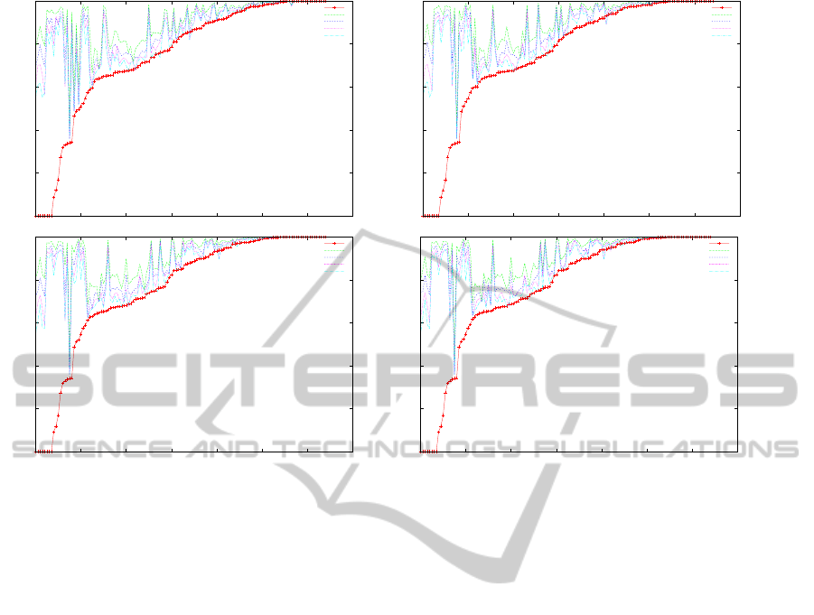
In the light of the results (Figure 6), this smoted
technique produce incredibly good results for all clas-
sifiers. For space problems, we do not show all the
classifiers, but we remark that the same tendency re-
peats for every classifier. There seem to be a particu-
lar dataset where using IR
′
3 and 4, performs slightly
worse than using the original IR. This is less than 1%
of our datasets. Furthermore, when IR
′
is 1 or 2, we
obtain much better results in all the datasets.
4.3 Conclusions from the Results
From the previous results, it is evident that the use
of smoted re-balancing provides incredibly good re-
sults for all datasets. Experimentation seems to rec-
ommend especially IR’ as 1 or 2. The decision about
this value can be taken depending on the importance
of using less times (IR2 will create less new minority
cases). However, time for small datasets is not impor-
tant, on average (for all tested models), evaluating the
four new IR values for one dataset takes around one
third of a second, in a relatively old computer (Java
on Intel(R) Core(TM)2 Duo CPU, 2.66GHz and 2GB
for RAM), and AODE is faster than this average.
The most important conclusions from our explo-
ration on BNCs in this representative (129) set of im-
balanced datasets could be summarised as follows:
• All BNCs performed much better in imbalanced
data than decision trees (C4.5), one of the tested
models in previous papers.
• Among BNCs, Naive Bayes does not work
bad, but the conditional independence assumption
makes the model too simple and it provides lower
performance for some datasets.
• AODE seems to provide the better results, since
more complex semi-Naive Bayes, as kDB or TAN
do not obtain better results, in terms of AUC.
• Our proposal, based on smoted re-balancing, out-
performs the original results very significantly.
5 FINAL DISCUSSION
In this work we have performed a study on how
Imbalance Ratio affects when using Bayesian Net-
works models in classifying, when the dataset from
which the model is learned presents imbalance be-
tween classes. As seen in the introduction, this prob-
lem is quite frequent in certain fields. We have seen
that this relation IR with performance is not trivial,
and cannot be caught with a linear function, as many
other factors, intrinsic in the dataset can affect, as dis-
cussed in (Lopez et al., 2013). However, working
with this IR in combination with over-sampling tech-
niques, as SMOTE, can produce an incredible gain in
the classification assessment. So, the two main con-
tributions of this paper is the use of BNCs for imbal-
anced datasets together with analysis of their perfor-
mance in a public benchmark with 129 datasets, and
the proposal of a new algorithm in which we recom-
mend to use AODE as classifier and IR’ as 1 or 2,
but which could be parametrised with other BNC and
value and will work properly depending on the user
preferences.
As future work there are two possible lines: inves-
tigate sophisticated boosting techniques focused on
imbalanced dataset that use cost functions (Sun et al.,
2007), probably with some adaptation to BNCs, and
also, the use of other oversampling methods distinct
ICAART2015-InternationalConferenceonAgentsandArtificialIntelligence
388
0.5
0.6
0.7
0.8
0.9
1
0 20 40 60 80 100 120 140
Orig
IR1
IR2
IR3
IR4
0.5
0.6
0.7
0.8
0.9
1
0 20 40 60 80 100 120 140
Orig
IR1
IR2
IR3
IR4
0.5
0.6
0.7
0.8
0.9
1
0 20 40 60 80 100 120 140
Orig
IR1
IR2
IR3
IR4
0.5
0.6
0.7
0.8
0.9
1
0 20 40 60 80 100 120 140
Orig
IR1
IR2
IR3
IR4
Figure 6: For each classifier, datasets are set in the x-axis in an ascending order with respect to original AUC value. Top left:
NB Discrete; Top right: AODE; Bottom left: 2DB; Bottom right: 3DB. y-axis range is 0.5 to 1.
from SMOTE. Finally, we aim at studying algorithms
to learn BNCs tailored for imbalanced data. The ex-
tension to multi-class problem could also be useful.
ACKNOWLEDGEMENTS
This work has been partially funded by FEDER
funds and the Spanish Government (MINECO) un-
der projects TIN2010-20900-C04-03 and TIN2013-
46638-C3-3-P.
REFERENCES
Breiman, L. (1998). Arcing classifiers. Annals of Statistics,
26:801–823.
Chawla, N., Bowyer, K., Hall, L. O., and Kegelmeyer, W. P.
(2002). SMOTE: Synthetic Minority Over-sampling
TEchnique. Journal of Artificial Intelligence Research
(JAIR), 16:321–357.
Fayyad, U. M. and Irani, K. B. (1993). Multi-interval dis-
cretization of continuous valued attributes for classi-
fication learning. In Thirteenth International Joint
Conference on Artificial Intelligence, volume 2, pages
1022–1027. Morgan Kaufmann Publishers.
Flores, M. J., G´amez, J. A., and Mart´ınez., A. M. (2012).
Supervised classification with Bayesian networks: A
review on models and applications., chapter 5, pages
72–102. IGI Global.
Flores, M. J., G´amez, J. A., Mart´ınez, A. M., and Puerta,
J. M. (2011). Handling numeric attributes when com-
paring bayesian network classifiers: does the dis-
cretization method matter? Applied Intelligence,
34(3):372–385.
Huang, J. and Ling, C. X. (2005). Using auc and accuracy
in evaluating learning algorithms. IEEE Transactions
on Knowledge and Data Engineering, 17(3):299–310.
Kononenko, I. (1991). Semi-naive bayesian classifier. In
Machine Learning EWSL-91, volume 482 of Lecture
Notes in Computer Science, pages 206–219.
Korb, K. B. and Nicholson, A. E. (2010). Bayesian artificial
intelligence. Chapman & Hall/CRC, 2nd edition.
Lopez, V., Fernandez, A., Garcia, S., Palade, V., and Her-
rera, F. (2013). An insight into classification with im-
balanced data: Empirical results and current trends on
using data intrinsic characteristics. Information Sci-
ences, 250(0):113 – 141.
Sun, Y. (2007). Cost-sensitive boosting for classification of
imbalanced data. PhD thesis, Department of Electri-
cal and Computer Engineering, University of Water-
loo.
Sun, Y., Kamel, M. S., Wong, A. K. C., and Wang, Y.
(2007). Cost-sensitive boosting for classification of
imbalanced data. Pattern Recognition, 40(12):3358–
3378.
Wasikowski, M. and wen Chen, X. (2010). Combating the
small sample class imbalance problem using feature
selection. Knowledge and Data Engineering, IEEE
Transactions on, 22(10):1388–1400.
Webb, G. I., Boughton, J. R., and Wang, Z. (2005). Not so
naive bayes: Aggregating one-dependence estimators.
Machine Learning, 58(1):5–24.
ImpactonBayesianNetworksClassifiersWhenLearningfromImbalancedDatasets
389
