Vessel Rotation Planning

A Layered Distributed Constraint Optimization Approach

Shijie Li, Rudy R. Negenborn and Gabriel Lodewijks

Faculty of Mechanical, Maritime and Materials Engineering,

Delft University of Technology, Mekelweg 2, 2628 CD Delft, The Netherlands

Keywords:

Multi-agent Systems, Constraint Optimization, Planning and Scheduling.

Abstract:

Vessel rotation planning concerns the problem of assigning rotations to vessels over a number of terminals for

loading and unloading containers in a large port. Vessel operators and terminal operators communicate with

each other to make appointments about the rotation plans for the vessels. However, it happens frequently that

these appointments cannot be met. Thus, it is important to generate the rotation plans for the vessel operators

in an efﬁcient automated way. In this paper, we propose an approach to solve the vessel rotation planning

problem by modeling the problem as a layered distributed constraint optimization problem (DCOP). To

evaluate the performance of the proposed approach, combinations of three DCOP algorithms are considered,

namely, Asynchrounous Forward Bounding, Synchrounous Branch and Bound, and Dynamic Programming

Optimization Protocol. We evaluate the solution quality and computational and communication costs of these

three algorithms when solving the vessel rotation planning problem using the proposed layered formulation.

1 INTRODUCTION

A vessel rotation is the sequence in which a vessel

visits different terminals in a large port. The

vessel rotation planning problem (VRPP) concerns

the problem of assigning rotations to a number

of vessels over a number of terminals that they

have to visit. The decision makers involved are

vessel operators and terminal operators. Vessel

operators are responsible for the voyage plan of

vessels and coordinating inland shipping activities,

while terminal operators are responsible for the

transshipment of containers between deep sea vessels,

trains, trucks, and inland vessels as well as the

temporary storage of containers. As an example, on

a typical day, around 25 inland vessels visit the Port

of Rotterdam, and each vessel visits on average 8

different container terminals (Moonen et al., 2007).

Nowadays, vessel operators and terminal opera-

tors communicate with each other through telephone,

fax and e-mail for making appointments. However,

in practice, the appointments made often cannot be

met (Melis et al., 2003). In the port of Rotterdam,

the average rotation time for an inland vessel is

approximately 22.5 hours, of which only 7.5 hours

are used for loading and unloading, the rest of the

time vessels are waiting and traveling (Moonen et al.,

2007). A disturbance at one terminal can lead to the

interruption of the operations of a vessel and terminal

operators elsewhere. This can make it difﬁcult for

vessel operators to stick to the appointments made

with terminal operators (Douma, 2008).

There have been several publications on the

alignment of vessels and terminals in recent years.

In (Schut et al., 2004), a multi-agent based and

distributed planning system named APPROACH has

been introduced. The outcomes of the software

sometimes, however, contained routes considered

unlogical and with longer sailing times than needed

(Moonen et al., 2007). In (Douma et al., 2009)

the same type of agents is used but with different

interaction protocols and agent structure. The authors

improve the multi-agent systems by considering de-

sign choices that could inﬂuence the acceptance of the

end users and the extent to which users can optimize

their operations in (Douma et al., 2012).

The problem considered in this paper consists of

ﬁnding in an automated way the best solution to a

VRPP rotation plan for a given set of vessels. Our ap-

proach proposes to use layered distributed constraint

optimization (DCOP). DCOP is a theoretical model

framework where several agents communicate with

each other to take on values so as to minimize the

sum of the resulting constraint costs. In (Li et al.,

166

Li S., R. Negenborn R. and Lodewijks ..

Vessel Rotation Planning - A Layered Distributed Constraint Optimization Approach.

DOI: 10.5220/0005202801660173

In Proceedings of the International Conference on Agents and Artiﬁcial Intelligence (ICAART-2015), pages 166-173

ISBN: 978-989-758-073-4

 2015 SCITEPRESS (Science and Technology Publications, Lda.)

2014), we made the a ﬁrst proposal for using DCOP

for the VRPP. In this paper, we extended this work

ﬁrstly proposing a layered DCOP structure that splits

the rotation planning process into two layers so that

relatively large problem instances can be considered;

secondly, we propose a different model from (Li

et al., 2014); we introduce waiting time variable in

the objective function, so that the ﬁnal rotation plans

include the arrival, waiting, departure and travel time

of each vessel, which makes the model more realistic;

thirdly, the performance of combinations of three

DCOP algorithms are compared with respect to the

communication load and simulated time.

This paper is organized as follows. In Section 2,

the deﬁnitions for DCOP and VRPP are introduced.

In Section 3, the VRPP is deﬁned and formulated

as layered DCOP and solution algorithms are in-

troduced. Section 4 presents the implementation

of the proposed approach and experimental results.

Conclusions and future work are given in Section 5.

2 DCOP AND LAYERED DCOP

2.1 Distributed Constraint

Optimization Problems

We use the DCOP formalism as deﬁned in (Petcu,

2009). A DCOP is represented by a triple

hA, C OP , R

i, where, A = {A

, . . . , A

} is a

set of N agents; C OP = {COP

, . . . , COP

} is a set

of disjoint, local Constraint Optimization Problems

(COPs); COP

is called the local sub-problem of

agent A

, and has to be solved by agent A

; COP

is a

triple hX

, D

, R

i, where X

is a set of variables that

belongs to A

; D

is a set of ﬁnite variable domains;

is a set of utility functions, which can also be used

to represent objectives, hard and soft constraints;

= {r

, . . . , r

} is a set of inter-agent utility

functions deﬁned over variables of multiple agents.

Each r

: scope(r

) → R expresses the utility for

joint decision obtained by the agents that have

variables involved in r

. The agents involved in r

can decide on the values of the variables involved.

The objective of the agents solving a DCOP is

to ﬁnd the assignments to all variables X

∗

such that

all the constraints are satisﬁed (expressed via utility

functions) and the sum of values of all the utility

functions representing the objectives is maximized,

∗

= arg max

∑

i=1

∑

v=1

, . . . , X

i|X

)

∑

l=1

To ﬁnd the optimal solution X

∗

, agents need to

communicate and exchange messages that include

information on the assignments of values to variables

and the related utility values among each other. Thus,

the total number of messages and the size of messages

sent by the agents is an important performance metric

for measuring the efﬁciency of DCOP algorithms.

Based on the completeness of the algorithms,

DCOP algorithms can be categorized as complete

and incomplete algorithms. Complete algorithms

typically do an exhaustive search over the problem

space: thus, they can guarantee ﬁnding an optimal

solution, while incomplete algorithms usually use

local search methods to ﬁnd locally optimal solutions,

and thus can potentially get trapped in local minima

or fail to converge to any solution altogether. In

(Petcu, 2009), a detailed description and comparison

of the DCOP algorithms can be found. In this paper,

we compare the performances of the combinations of

three different complete algorithms, including DPOP,

AFB and SyncBB.

2.2 Layered DCOP

As solving DCOP problems is NP-hard (Modi et al.,

2005), increasing the number of variables increases

the complexity of the problem exponentially. There-

fore, using straightforward DCOP methods for solv-

ing VRPPs that consist of many vessels and terminals

brings high computation and communication costs.

Partitioning of the DCOP could signiﬁcantly improve

the solution process.

In (Hosseini et al., 2013), the authors consider

a hierarchical DCOP setting for a target to sensor

allocation problem, in which they change the orig-

inal DCOP as a hierarchical set of smaller DCOPs

with shared constraints in order to avoid signiﬁcant

computational and communication costs. The results

show that compared with a non-hierarchical structure,

the hierarchical modeling technique provides superior

results, with the advantage becoming more signiﬁcant

under increased problem size and complexity.

Using a partitioned method prevents the creation

of large DCOPs, potentially reducing the compu-

tational complexity greatly (Hosseini et al., 2013),

although this can also be at the cost of lower solution

quality. Thus, in this paper we propose a layered

structure for the VRPP formulated as DCOP so

that the computation and communication costs can

be reduced. We split VRPP into two layers of

DCOPs, the solutions from the upper layer will be the

constraints in the lower layer. On the upper layer is

the DCOP that involves all the vessels, while in the

lower layer, there are sets of smaller DCOPs, each

vessel having 1 DCOP.

VesselRotationPlanning-ALayeredDistributedConstraintOptimizationApproach

167

3 LAYERED DCOP FOR VESSEL

ROTATION PLANNING

3.1 Vessel Rotation Planning Problem

VRPP concerns selecting the rotation plan consisting

of sequences and arrival and departure times of

vessels to terminals in a port area. To model the VRPP

as a DCOP, we make the following assumptions:

• Decisions are made at discrete time steps, so

discrete time slots can be considered.

• Each vessel knows which terminals it needs to

visit. The visiting sequence, is unknown. Each

vessel has its own preference over the visiting

sequence for different terminals.

• Distances between terminals are given.

• Service time of a vessel at a terminal is known.

The problem can now be formalized using the follow-

ing variables:

• A set of vessels: V = {1, 2, 3, ..., N}

• A set of terminals: T = {1, 2, 3, ..., M}

• A set of discrete time slots: D = {1, 2, 3, ..., P}

• x

i j

represents the time slot at which vessel i is at

terminal j

• a

i j

, d

i j

and w

i j

represents the arrival, departure,

and waiting time of vessel i at terminal j, respec-

tively

We use the following parameters in our model:

• U

i j

represents the preference of vessel i of being

at terminal j during time slot k

• W

i j

represents the utility value of variable w

i j

• s

i j

represents service time of vessel i at terminal j

• t

represents traveling time from terminal m to n

• [T

k−1

, T

] is a ﬁxed time window for terminal j

when it is visited by vessels during time slot k

i j

is used to represent the preferences of vessel i

at terminal j. For example, U

= 5, U

= 4, U

= 3

means that vessel 1 prefers to visit terminal 1 during

time slot 1, since it has the highest utility value. These

utilities are implemented in the DCOP framework by

assigning different preference values (utility values

that represents the preference of vessels) when x

i j

= k,

and assigning 0 to all the situation when x

i j

6= k.

i j

is used to represent the utility value for w

i j

k. A higher value of k represents a longer waiting time

of vessel i at terminal j. Thus, the higher the value of

k is, the lower the value of W

i j

will be. Service time

i j

and traveling time t

are integer constants.

k−1

, T

] is a ﬁxed time window for terminal j

when it is visited by vessels during time slot k, for

example, [T

, T

] = [6, 10] means that if vessel i visit

terminal 1 during time slot 3, the arrival time of vessel

i at terminal 1 must be within the time window [6, 10].

We introduce the concept of time window to ensure

that for the vessel that visits terminal j during time

slot k, it can be serviced only if it arrives at the

terminal within a speciﬁed time window [T

k−1

, T

is the deadline for a vessel’s arrival to be serviced

at terminal j if it visits the terminal during time slot k.

The objective is to ﬁnd the optimal rotation

plan for vessels, which includes the sequences and

departure and arrival time at each terminal, such that

a set of utility functions are maximized.

3.2 Agents Structure

VRPP can be modeled as a DCOP by considering the

vessels as agents, the constraints related with vessels

as constraints of local problems of the agents. As

the constraints for terminals usually involve variables

from different vessel agents, these constraints can

considered as inter-agent utility functions. In our

model, agent A

represents vessel i. In the local

problem of A

, values of variables x

i j

, a

i j

, d

i j

and w

i j

are determined by A

. The inter-agent and local utility

functions are deﬁned as hard constraints related to a

vessel i. The preference of vessels at terminals during

different time slots are also considered as the utilities

of the local COPs of the vessel agents.

For the DCOP we will formulate, the objective

is ﬁnd the assignments of values from domain D to

variables x

i j

, a

i j

, d

i j

and w

i j

, that maximizes the sum

of values of the utility functions of local COPs and the

inter-agent utility functions. The inter-agent utilities

are represented as the terminal capacity constraints.

Based on the above structure, we can provide a

general deﬁnition of the VRPP as DCOP, as a tuple of

the following form, hA , C OP , R

i, in which A is the

set of vessel agents; C OP is the set of local constraint

optimization problems for each vessel agent; R

the set of inter-agent utility functions deﬁned over

variables from different vessel agents.

3.3 Layered DCOP for VRPP

Problem solving using a layered structure uses a top

down approach. As we can see from Figure 1, the

upper layer is what we deﬁne as assignment problem,

which decides the sequence in which the vessels visit

different terminals. When the solutions have been

obtained at the higher layer, the lower layer, which we

deﬁne as scheduling problem, will decide the exact

arrival, departure and waiting time of each vessel at

each terminal. There is one DCOP in the upper layer

ICAART2015-InternationalConferenceonAgentsandArtificialIntelligence

168

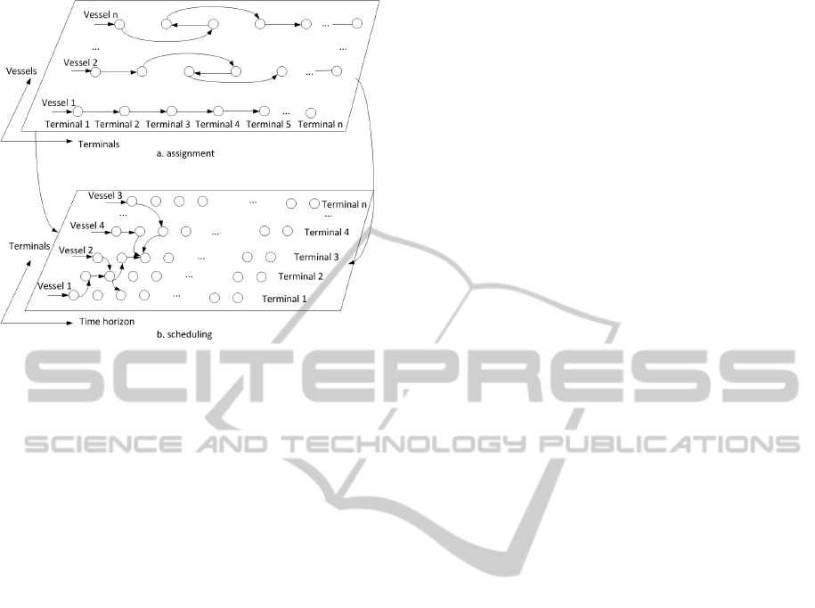
Figure 1: Layered DCOP structure.

that relates to all the vessels, while there are multiple

smaller DCOPs in the lower layer, each relating only

to 1 vessel. After ﬁnding an optimal solution for the

upper layer DCOP problem, the lower layer’s DCOP

solver starts solving each problem separately. There

are common variables between the upper layer DCOP

and the lower layer DCOPs. In solving the problem

of the lower layer, the algorithm is not concerned with

the values maintained by the upper layer, but only

with the solutions obtained from upper layer.

3.3.1 Assignment Problem

At the upper layer, we only consider the sequence of

vessels’ visits to terminals. Thus, only variable x

i j

which represents the time slot at which vessel i is at

terminal j is involved. The exact arrival, departure

and waiting time of vessels will not be included in

this layer; these are considered in the lower layer.

The local COP

of A

is deﬁned by a triple

, D

, R

i. Here, X

= {x

, . . . , x

i|X

} is a

set of variables, in which x

i j

represents the time

slot at which vessel i is at terminal j; D

, . . . , d

i|D

} is a set of ﬁnite variable domains,

for each d

i j

∈ {1, 2, 3, ..., P}; R

= {r

, . . . , r

i|R

}

contains utility functions that represent the constraints

related with vessels and the their preferences over

different terminals during different time slots. Thus,

we have,







i j

: ifx

i j

= k ∀i ∈ {1, 2, ..., N},

∀ j ∈ {1, 2, ..., M}, k ∈ {1, 2, ..., P}

0 : otherwise

(1)







0 : all-different(x

, . . . , x

)

∀i ∈ {1, 2, ..., N}

−∞ : otherwise

(2)

Utility function r

represents the preferences of

vessel i being at terminal j during time slot k. U

i j

is a constant deﬁned for different combinations of i,

j and k. Utility function r

is deﬁned based on the

all-different constraint as in (Rossi et al., 2006), it

uses the all-different constraint to ensure that each

vessel will only be at most at one terminal during a

time slot.

In addition, we deﬁne the inter-agent utility

functions as the capacity constraints of terminals,

i.e. each terminal can serve only a limited num-

ber of vessels simultaneously. We incorporate the

cumulative constraint from constraint programming

to represent the inter-agent utility functions r

ia,as

the assignment problem,

ia,as







0 : cumulative((x

1 j

, . . . , x

N j

), s

i j

, 1, N

)

∀ j ∈ {1, 2, ..., M}

−∞ : otherwise

(3)

In which, (x

1 j

, . . . , x

N j

) are the variables repre-

senting time slots at which the vessels that will be

at terminal j. s

i j

is the service time for a vessel

at a terminal. Consumption rate c is set to 1

because a vessel will be serviced by one terminal.

is the number of vessels one terminal can serve

simultaneously.

For the overall DCOP assignment problem, the

objective is to maximize the sum of values of

individual utility functions and the inter-agent utility

functions, deﬁned as:

max

∑

i=1

+ r

) + r

ia,as

(4)

3.3.2 Scheduling Problem

When the solutions x

i j

from the assignment prob-

lem have been obtained, we can determine the

sequence of vessels to different terminal j and

the time slots during which each vessel will be

at terminals. We can formulate the scheduling

problem based on DCOP similar to the assignment

problem as a tuple hA

, C OP

, R

ia,sc

i. The lo-

cal problem COP

of each vessel agent A

deﬁned by a triple hX

, D

, R

i, where, X

, . . . , a

i|X

, d

, . . . , d

i|X

, w

, . . . , w

i|X

} is a set

of variables, and a

i j

, d

i j

represent the arrival, depar-

ture time of vessel i from terminal j, w

i j

represents

the waiting time of vessel i at terminal j; D

, . . . , k

i|D

}is a set of variable domains, for each

i j

∈ {1, 2, 3, ..., P}; R

= {r

, . . . , r

i|R

} contains

utility functions that represent the constraints for

vessels’ arrival, departure and waiting at terminals.

VesselRotationPlanning-ALayeredDistributedConstraintOptimizationApproach

169

The inter-agent utility function r

ia,sc

for the

scheduling problem is deﬁned as follows:

ia,sc

(

0 : if x

= x

+ 1, then a

= d

∀i ∈ {1, 2, ..., N}, ∀m, m

∈ {1, 2, ..., M}

−∞ : otherwise

(5)

ia,sc

ensures that if vessel i travels from terminal

m to m

, the arrival time at terminal m

is the sum of

departure time from m and the traveling time t

For each vessel agent, we have the utility func-

tions as follows (for the following constraints we have

k, k

∈ {1, 2, 3, ..., P}),







0 : if x

i j

= k, then a

i j

∈ [T

k−1

, T

]

∀i ∈ {1, 2, ..., N}, ∀ j ∈ {1, 2, ..., M}

−∞ : otherwise

(6)







0 : if d

i j

= a

i j

+ w

i j

+ s

i j

∀i ∈ {1, 2, ..., N}, ∀ j ∈ {1, 2, ..., M}

−∞ : otherwise

(7)







0 : if x

i j

= k, then w

i j

= T

− a

i j

∀i ∈ {1, 2, ..., N}, ∀ j ∈ {1, 2, ..., M}

−∞ : otherwise

(8)







i j

: ifw

i j

= k

∀i ∈ {1, 2, ..., N},

∀ j ∈ {1, 2, ..., M}

0 : otherwise

(9)

Utility function r

ensures that if vessel i visits

terminal j during time slot k, the arrival time should

be within the time window [T

k−1

, T

] of time slot k. If

vessel i cannot arrive within the time window, it will

not be serviced during time slot k and has to wait to

be serviced during the next time slot.

Utility function r

ensures that the departure time

of a vessel from a terminal equals the sum of the

vessel’s arrival time, waiting time and service time

at the terminal. Utility function r

ensures that the

waiting time is the difference between the arrival time

of a vessel i at terminal j and the start time for the

vessel to be serviced at the terminal.

Utility function r

ensures that the shorter the

waiting time w

i j

is, the higher the utility value W

i j

will be. This utility is used to make sure that the

objective of maximization of the sum of utility values

will lead to the minimization of the sum of waiting

times. As we can see, r

, r

ia,sc

depends on the

solutions for x

i j

from the assignment problem.

The objective is to maximize the sum of the values

of the individual utility functions and the inter-agent

utility functions, deﬁned as:

max

∑

i=1

+ r

) + r

ia,sc

(10)

3.4 Solution Algorithms

In this section, we will use DPOP introduced by

(Petcu and Faltings, 2005a) as an example to illustrate

the mechanism of solving vessel rotation planning

problem based on DCOP.

Firstly, a depth ﬁrst search (DFS) structure is

established using a distributed DFS algorithm. Each

variable is considered as a node. Each agent controls

a set of variables. The nodes consistently label

each other as parent/child nodes, and the edges are

identiﬁed as tree/back edges. In our case, agent

and agent A

represent the same vessel i in

the assignment problem and scheduling problem,

respectively. This means that variables x

i j

are owned

by A

, while a

i j

, d

i j

and w

i j

are owned by A

The second phase is UTIL propagation, the objec-

tive of which is to propagate aggregated utilities up

the DFS tree. Initially, messages travel up in the DFS

tree, propagating information about the aggregated

optimal costs/utilities. For example, for each variable

i j

belonging to agent A

, agent A

joins the

constraints involving x

i j

together, while ignoring all

constraints that involve at least one descendant of x

i j

Then agent A

waits for the reception of a UTIL

message from each of the child nodes of x

i j

, and

joins them all together with its constraints. Finally,

agent A

eliminates x

i j

from the join, and sends the

resulting utility to the parent node of x

i j

. This utility

corresponds to the maximum achieved utility for the

whole subtree rooted at x

i j

, as a function of the value

for the parent node of x

i j

and also the values for other

variables higher than x

i j

in the DFS tree.

The third phase of DPOP is VALUE propagation.

At the end of the UTIL propagation, the root variable

has obtained its own local optimal value based on

the messages it received. The agent that controls the

value of the root variable sends this optimal value to

each of the child nodes of the root variable through

VALUE messages. Recursively, for each variable x

i j

when the corresponding agent receives the VALUE

message from the parent node of that variable x

i j

, is

able to look up its own corresponding optimal value

during the UTIL propagation phase. To each of the

children nodes of x

i j

, agent A

sends not only the

optimal value of x

i j

, but also the optimal values for all

the variables in x

i j

’s children node’s separator(parent

and pseudo-parents nodes), which are contained in

the VALUE message it receives. Optimal decisions

are hereby propagated down the DFS tree, until all

variables have been assigned optimal values.

SyncBB and AFB are alternative DCOP algo-

rithms that use a linear ordering of agents instead

of a DFS tree. For SyncBB, at each step an agent

ICAART2015-InternationalConferenceonAgentsandArtificialIntelligence

170

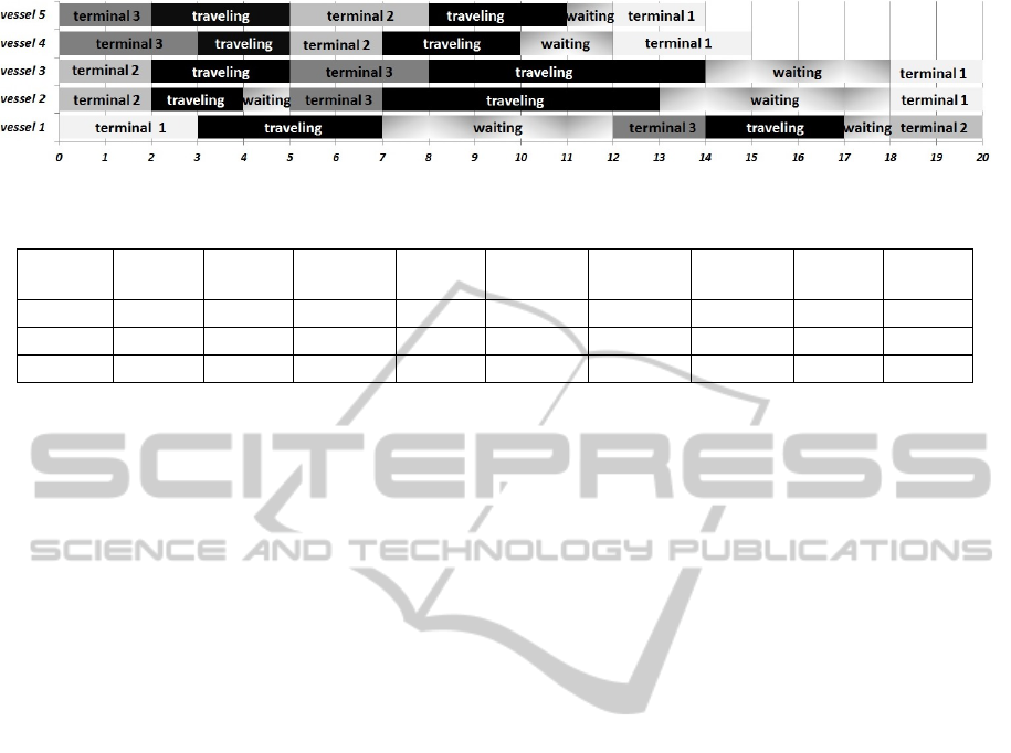
Figure 2: Rotation plan (5 vessels, 3 terminals)

Table 1: Comparison of the total number of messages for different cases and algorithms (by type)

DPOP+

DPOP

AFB+

AFB

SyncBB+

SyncBB

DPOP+

SyncBB

+ DPOP

AFB +

SyncBB

SyncBB+

AFB

DPOP+

AFB

AFB +

DPOP

Case 1

127 4,923 4,685 2,013 2,815 4,746 4,853 2,574 2,885

Case 2

307 14,562 11,559 3,509 8,357 12,412 13,706 5,659 9,120

Case 3

392 24,132 23,520 4,650 8,927 21,230 22,964 6,752 10,237

* The total number of messages exchanged is the same for the three different tests of the same case.

tries to assign a value to the current assignment

without causing the lower bound to reach the upper

bound while for AFB, agents perform asynchronous

concurrent checks of bounds. More details of

SyncBB and AFB are given in (Gershman et al.,

2009) and (Hirayama and Yokoo, 1997).

4 EXPERIMENTS

The DCOP algorithms we experiment with are imple-

mented in the FRODO2 toolbox (L

eaut

e et al., 2009).

Our tests are performed on an Intel Core i5-2400 CPU

with RAM 4GB under Windows 7. Values reported

here are averages of 10 repetitions of the simulation.

4.1 Setup

To test the effectiveness of the DCOP algorithms,

we choose 3 different types of DCOP algorithms, in-

cluding DPOP, AFB and SyncBB. We apply different

algorithms in the two layers, the assignment problem

and the scheduling problem. In order to evaluate the

communication load and simulated time of the three

algorithms, three performance metrics are measured:

total number of messages, total size of messages, and

average simulated time.

We also differ cases concerning the number of

vessels and terminals. We summarize this below:

• Case 1: 3 vessels, 3 terminals, each vessel needs

to visit 3 terminals, 36 variables, 55 constraints;

• Case 2: 5 vessels, 3 terminals, each vessel needs

to visit 3 terminals, 60 variables, 93 constraints;

• Case 3: 7 vessels, 5 terminals, each vessel needs

to visit 3 terminals, 80 variables, 157 constraints.

For each case, we choose 10 different groups of

values for U

i j

and W

i j

. Thus, we run 30 experiments

in total. The range of the utility value for U

i j

and W

i j

is arbitrary in our tests, but higher value means higher

priority. In addition, we assume that one terminal can

serve two vessels simultaneously (N

= 2).

4.2 Results

4.2.1 Generated Schedule Plan

Based on the solutions we have obtained from the

experiments, we can get the arrival time, departure

time, service time and travel time for each vessel from

variable a

i j

, d

i j

, s

i j

and t

, respectively. Due to space

limitations, here we only present one of the rotation

plans generated using DPOP in both assignment and

scheduling problem in the Case 2 as an example,

which is shown in Figure 2. The ﬁgure shows the

rotation plan for 5 vessels, and 3 terminals. In this

ﬁgure, different colors represent different terminals.

As we can see, when a vessel does not arrive at the

terminal within the corresponding time window, it has

to wait at the terminal until the next available time

window of the terminal. From this rotation plan, each

vessel operator can determine the sequence in which

to visit the different terminals and exact arrival and

departure time.

4.2.2 Communication Load

Table 1 and Table 2 show the comparison of total

number of messages and size of messages. The

number and size of messages calculated here include

both the inter-agent and intra-agent messages. With

respect to the total number of messages, applying only

the DPOP algorithm results in the lowest number of

VesselRotationPlanning-ALayeredDistributedConstraintOptimizationApproach

171

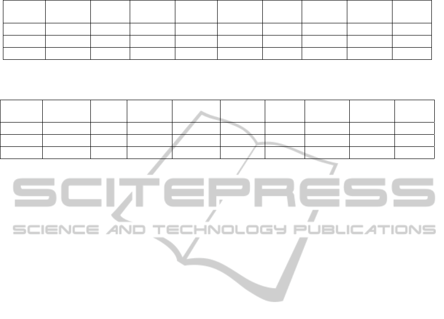
Table 2: Comparison of the total size of messages for different cases and algorithms (/bytes).

DPOP +

DPOP

AFB +

AFB

SyncBB+

SyncBB

DPOP+

SyncBB

SyncBB+

DPOP

AFB+

SyncBB

SyncBB+

AFB

DPOP+

AFB

AFB+

DPOP

Case 1

31,342 139,423 106,323 72,986 65,391 120,949 128,757 142,964 76,057

Case 2

5,927,266 726,259 265,855 6,009,593 183,528 471,473 520,641 6,264,379 389,146

Case 3

8,926,286 809,437 484,567 8,462,975 2,987,432 575,984 620,453 8,764,275 487,276

* The total size of messages exchanged is the same for the three different tests of the same case.

Table 3: Comparison of average simulated time for different cases and algorithms (/ms).

DPOP+

DPOP

AFB+

AFB

SyncBB+

SyncBB

DPOP+

SyncBB

SyncBB+

DPOP

AFB+

SyncBB

SyncBB+

AFB

DPOP+

AFB

AFB+

DPOP

Case 1

61 64 110 86 108 59 115 89 57

Case 2

2,352,094 163 343 2,352,130 298 165 341 2,352,114 120

Case 3

6,361,192 280 395 6,308,543 354 290 451 6,254,391 357

* The simulated time is the average of calculations based on all three tests for each case.

messages generated in all three cases. The reason is

that the number of messages is linear in the number

of agents and depends on the height of the DFS tree

associated with the problem being modeled (Petcu

and Faltings, 2005b). When the number of variables

and agents increase, the total number of messages

generated increases linearly. For all three cases, AFB

generate the largest number of messages.

However, with respect to the size of messages, the

situation is different. For small size problem as in

Case 1, DPOP has much smaller size of messages

than the others, however, with the increase of agents

and variables, the size of messages for DPOP increase

exponentially, while for AFB and SyncBB, the size

of messages does not increase as signiﬁcantly as

DPOP as in Case 2 and Case 3. The reason is that

complexity of DPOP is given by the size of the largest

UTIL message it produces, aggregated from the

communication between parent agents and children

agents in the DFS tree, which is exponential in the

induced width of the DFS ordering used. Thus, DPOP

sends out exponentially larger messages (but only a

linear number of them), while the other algorithms

send out an exponential amount of messages but of

only linear size.

4.2.3 Simulated Time

Table 3 shows the simulated time of DCOP algo-

rithms. For smaller cases like Case 1, the simu-

lated time for each algorithm does not differ much.

SyncBB has slightly longer simulated time. However,

with the increase of problem size, in Case 2 and Case

3, DPOP has the longest simulated time in either

the upper layer or the lower layer. For SyncBB and

AFB, the simulated does not have steep increases

as for DPOP. AFB has a shorter simulated time

than SyncBB. This happens because the memory

requirement for DPOP is exponential in the induced

width of the DCOP problem, which depends on the

number of backedges (the links between nodes and

their pseudo-parents) in the DFS tree (Petcu and

Faltings, 2005b). It can be as large as the number

of agents minus one of the constraint graph is fully

connected and every agent is thus constrained with

every other agent. For SyncBB and AFB, the memory

requirements are polynomial in the number of agents.

To conclude, DPOP outperforms AFB and

SyncBB in the total number of messages exchanged.

However, this performance is achieved with a high

increase in message size and simulated time (the

growth of which is exponential in the DFS tree-

width) which makes it inapplicable to DCOPs with

large tree-widths and larger problem sizes. Our

results suggest that SyncBB offers the best tradeoff

between communication load and simulated time on

this problem class. These results seem to indicate

that AFB is not the best suited algorithm for the

VRPP. This could be due to the problem’s variety and

complexity.

5 CONCLUSIONS AND FUTURE

RESEARCH

This paper proposes a new method for solving the

vessel rotation planning problem using a DCOP ap-

proach. We use a non-binary variable representation

to reduce the number of variables and constraints,

and incorportate a layered structure to divide the

main problem into smaller ones and simplify the

complex and hard problem. Three DCOP algorithms

are compared over three different cases. Results

ICAART2015-InternationalConferenceonAgentsandArtificialIntelligence

172

show that it is possible to verify the effectiveness

and efﬁciency of DCOP algorithms in the proposed

application.

To take the DCOP approach into application,

the problem size should at least be increased to 22

vessels, 8 terminals. In addition, the constraints from

the perspective of terminal operators should be taken

into consideration for future work.

Although the layered problem solving decreases

computation and communication cost , addressing

the problem in a layered way may lead to ﬁnding

sub-optimal solutions. The reason is that some

values are selected for the common variables in the

upper level and these selections may impose extra

constraints on these common variables in the lower

layer DCOPs. Lower layer DCOP then have to

keep previously selected values unchanged. On the

hand, considering the reduction of communication

and computation complexity of the layered approach,

in dynamic situations when DCOP algorithms do

not have enough time to reach the optimal solution,

the beneﬁt of using a layered approach strongly

outweighs its costs drawback.

ACKNOWLEDGEMENTS

This research is supported by the China Scholarship

Council under Grant 201206680009 and the VENI

project “Intelligent multi-agent control for ﬂexible

coordination of transport hubs” (project 11210) of the

Dutch Technology Foundation STW, a subdivision

of the Netherlands Organization for Scientiﬁc Re-

search (NWO). The authors would also like to thank

Dr.Thomas L

eaut

e for his constructive suggestions

regarding FRODO2 toolbox.

REFERENCES

Douma, A. (2008). Aligning the operations of barges and

terminals through distributed planning. PhD thesis,

University of Twente, Enschede, The Netherlands.

Douma, A., Schutten, M., and Schuur, P. (2009). Waiting

proﬁles: An efﬁcient protocol for enabling distributed

planning of container barge rotations along terminals

in the port of rotterdam. Transportation Research Part

C: Emerging Technologies, 17(2):133–148.

Douma, A., van Hillegersberg, J., and Schuur, P. (2012).

Design and evaluation of a simulation game to

introduce a multi-agent system for barge handling in a

seaport. Decision Support Systems, 53(3):465–472.

Gershman, A., Meisels, A., and Zivan, R. (2009).

Asynchronous forward bounding for distributed cops.

Journal of Artiﬁcial Intelligence Research, 34(1):61–

88.

Hirayama, K. and Yokoo, M. (1997). Distributed partial

constraint satisfaction problem. In Proceedings of

the 3rd International Conference on Principles and

Practice of Constraint Programming, pages 222–236.

Springer, Linz, Austria.

Hosseini, S., Samaneh, and Basir, O. A. (2013). Target to

sensor allocation: A hierarchical dynamic distributed

constraint optimization approach. Computer Commu-

nications, 36(9):1024–1038.

eaut

e, T., Ottens, B., and Szymanek, R. (2009).

FRODO 2.0: An open-source framework for dis-

tributed constraint optimization. In Proceedings of

the 21th International Joint Conference on Artiﬁcial

Intelligence, pages 160–164, Pasadena, California,

USA.

Li, S., Negenborn, R., and Lodewijks, G. (2014). A

distributed constraint optimization approach for vessel

rotation planning. In Proceedings of the 5th

International Conference on Computational Logistics,

pages 61–80, Valparaso, Chile.

Melis, M., Miller, I., Kentrop, M., Van Eck, B., Leenaarts,

M., Schut, M., and Treur, J. (2003). Distributed

rotation planning for container barges in the port of

rotterdam. Intelligent Logistics Concepts, pages 101–

116.

Modi, P. J., Shen, W.-M., Tambe, M., and Yokoo, M.

(2005). Adopt: Asynchronous distributed constraint

optimization with quality guarantees. Artiﬁcial

Intelligence, 161(1):149–180.

Moonen, H., Van de Rakt, B., Miller, I., Van Nunen,

J., and Van Hillegersberg, J. (2007). Agent

technology supports inter-organizational planning in

the port. Managing Supply Chains: Challenges and

Opportunities, pages 201–225.

Petcu, A. (2009). A class of algorithms for distributed con-

straint optimization. PhD thesis,

Ecole Polytechnique

erale de Lausanne, Lausanne, Switherland.

Petcu, A. and Faltings, B. (2005a). Approximations in

distributed optimization. In Principles and Practice of

Constraint Programming, pages 802–806. Springer.

Petcu, A. and Faltings, B. (2005b). A scalable method for

multiagent constraint optimization. In Proceedings of

the 19th International Joint Conference on Artiﬁcial

Intelligence, volume 5, pages 266–271, Edingurgh,

Scotland.

Rossi, F., Van Beek, P., and Walsh, T. (2006). Handbook of

constraint programming. Elsevier.

Schut, M. C., Kentrop, M., Leenaarts, M., Melis, M., and

Miller, I. (2004). Approach: Decentralised rotation

planning for container barges. In Proceedings of the

16th European Conference on Artiﬁcial Intelligence,

pages 755–759, Valencia, Spain.

VesselRotationPlanning-ALayeredDistributedConstraintOptimizationApproach

173