
Scheduling Problem in Call Centers with Uncertain Arrival Rates
Forecasts
A Distributionally Robust Approach
Mathilde Excoffier
1
, C
´
eline Gicquel
1
, Oualid Jouini
2
and Abdel Lisser
1
1
Laboratoire de Recherche en Informatique - LRI, Universit
´
e Paris-Sud, Orsay, France
2
Ecole Centrale Paris - ECP, Ch
ˆ
atenay-Malabry, France
Keywords:
Distributionally Robust Optimization, Stochastic Programming, Joint Chance Constraints, Mixed-Integer
Linear Programming, Staffing, Shift-Scheduling, Call Centers, Queuing Systems.
Abstract:
We focus on the staffing and shift-scheduling problem in call centers. We consider that the call arrival rates
are subject to uncertainty and are following unknown continuous probability distributions. We assume that we
only know the first and second moments of the distribution. We propose to model this stochastic optimization
problem as a distributionally robust program with joint chance constraints. We consider a dynamic sharing
out of the risk throughout the entire scheduling horizon. We propose a deterministic equivalent of the problem
and solve linear approximations of the program to provide upper and lower bounds of the optimal solution.
We applied our approach on a real-life instance and give numerical results.
1 INTRODUCTION
Call centers are the main interface between the firms
and their clients: in the U.S. in 2002, call centers
represent 70% of all business interactions (Brown
et al., 2005). Whether it be for emergencies call
centers or travel companies for example, the clients
are to be answered within a very limited time. The
Quality of Service is of prime importance in the
management of call centers. In addition, the staff
agents cost in call centers represents 60% to 80%
of the total operating budget (Aksin et al., 2007).
Thus firms have to propose a satisfying service while
controling the cost of the manpower. The importance
of this sector in the service economy and the practical
inherent constraints of the scheduling problem make
this problem a topical issue in Operations Research.
Practically, scheduling call centers consists in
deciding how many agents handling the phone calls
should be assigned to work in the forthcoming days
or weeks. The goal is to minimize the manpower cost
while respecting a chosen Quality of Service (QoS).
In call centers, we usually consider the expected
waiting time before being served, or the expected
number of clients hanging up before being served,
i.e. the abandonment rate, as a relevant measure of
Quality of Service.
The standard model for this problem is based
on forecasts of expected call arrival rates. These
forecasts are computed from historical data giving
the numbers of calls for the working time horizon.
Since the quantity of calls vary strongly in time, the
working horizon is split in small periods of time,
usually 30-minute periods. Thus we obtain for each
period an expected call arrival rate. Then we are able
to compute the staff requirements for each period
from the forecasts and an objective service level
which represents the chosen Quality of Service. This
computation is done with the well-known Erlang C
model. Finally, the numbers of agents required for
the whole working horizon are determined through
an optimization program, using the previous period-
by-period results.
The shift-scheduling problem presents some
characteristics: first, we need to split the horizon into
small periods of time in order to be able to represent
the variation of rate with the best precision possible.
This leads to an increasing number of variables.
Second, since we are considering human agents we
have to respect several manpower constraints. Thus,
agents have to follow established shifts and can not
work only for a few hours. Moreover, the solution
of the problem represents humans, so it has to be
integers. Finally, call arrival rates are forecasts and
thus subject to uncertainty. Thus, the final numbers
of agents computed is subject to uncertainty as well.
5
Excoffier M., Gicquel C., Jouini O. and Lisser A..
Scheduling Problem in Call Centers with Uncertain Arrival Rates Forecasts - A Distributionally Robust Approach.
DOI: 10.5220/0005203800050013
In Proceedings of the International Conference on Operations Research and Enterprise Systems (ICORES-2015), pages 5-13
ISBN: 978-989-758-075-8
Copyright
c
2015 SCITEPRESS (Science and Technology Publications, Lda.)

This should be considered in order to propose a valid
model.
Typical call centers models consider a queuing
system for which the arrival process is Poisson with
known mean arrival rates (Gans et al., 2003). Since
the data of the problem are forecasts of arrival rates,
the accuracy of this deterministic approach is lim-
ited. Indeed, these estimations of mean arrival rates
may differ from the reality. Uncertainty is taken into
account in several papers, with various approaches.
Several published works consider that input parame-
ters of the optimization program follow known distri-
butions. Some deal with continuous distributions (Ex-
coffier et al., 2014), discrete distributions (Luedtke
et al., 2007) or discretizations of a continuous distri-
bution into several possible scenarios (Robbins and
Harrison, 2010), (Liao et al., 2012) or (Gans et al.,
2012). However it can be difficult to estimate which
distribution is appropriate. (Liao et al., 2013) for call
centers and (Calafiore and El Ghaoui, 2006) for gen-
eral problems consider a distributionally robust ap-
proach. The problem deals with minimizing the fi-
nal cost considering the most unfavorable distribution
of a family of distributions whose parameters are the
given mean and variance. In (Liao et al., 2013), the
χ
2
statistic is used to build the class of possibles dis-
crete distributions, with a confidence set around the
estimated values. (Calafiore and El Ghaoui, 2006)
consider the set of radial distributions to characterise
the uncertainty region, but do not solve the final opti-
mization program for this set. Moreover they do not
focus on a specific problem and do not consider inte-
ger variables.
In the optimization program, we need to take into
account and manage the risk of not respecting the
objective service level. (Liao et al., 2012) and (Rob-
bins and Harrison, 2010) choose to penalize the non
respect of the objective service level with a penalty
cost in the objective function of the optimization
program. (Gurvich et al., 2010) and (Excoffier et al.,
2014) use a chance-constrained model, in which the
constraints are probabilities to be respected with the
given risk level. (Gurvich et al., 2010) focus on the
staffing problem but not the scheduling problem, and
consider only one period of time.
The contributions of this paper are the follow-
ing: first we model our problem with uncertain mean
arrival rates and a joint chance-constrained mixed-
integer linear program. This approach corresponds
well with the real requirements of the scheduling
problem in call centers. Indeed, forecasts are a use-
ful indication of what can happen in reality but can
not be considered as enough. This approach is in con-
trast with most previous publications whose risk man-
agement rely on a penalty cost. This penality can be
difficult to estimate.
Second we consider the risk level on the whole
horizon of study instead of period by period with joint
chance constraints. It enables to control the Quality
of Service on the whole horizon of study, which is
a critical benefit. Managers demand to have a weekly
vision of the call center, and not only for short periods
of time. Moreover we propose a flexible sharing out
of the risk through the periods in order to guarantee
minimization of the costs. As far as we know, this
consideration is only used in (Excoffier et al., 2014)
for the staffing and scheduling problem in call centers.
Finally we focus on a distributionally robust ap-
proach, considering that we only know the first two
moments of the continuous probability distributions.
Since we do not know in reality what is the ade-
quate distribution, we investigate a way of solving the
problem for unknown distributions. Unlike other pro-
posed distributionally robust approaches ((Liao et al.,
2013) in particular), we consider continuous distribu-
tions instead of discrete distributions. This allows to
a better representation of the reality. Moreover, (Liao
et al., 2013) focus on the uncertainty on the parame-
ters of a known gamma distribution whereas we focus
on the uncertainty of the distribution with known pa-
rameters.
The rest of the paper is organized as follows. In
Section 2 we present the formulation of the prob-
lem. At first, we propose the staffing model used
for computing the useful data of the scheduling prob-
lem. Then we introduce the distributionally robust
chance-constrained approach. In Section 3 we pro-
pose computations leading to the deterministic equiv-
alent of the distributionally robust program. We also
present the piecewise linear approximations leading
to the final programs whose solutions are lower and
upper bounds of the initial optimal solution. Section
4 gives an illustrative example of our approach. Fi-
nally in Section 5 we give numerical results.
2 PROBLEM FORMULATION
2.1 Staffing Model
The shift-scheduling problem is induced by the fact
that we consider whole number of human agents
working according to manpower constraints. We have
to consider that agents can not come and work for
only a few hours and need to follow working shifts
of full-time or part-time jobs. These shifts are made
ICORES2015-InternationalConferenceonOperationsResearchandEnterpriseSystems
6

up of working hours and breaks, for lunch for exam-
ple. The problem is then to decide how many work-
ing agents need to be assigned to each shift in the call
center in order to respect a choosen objective service
level. This computation uses data of calls arrival rates.
As previously explained, since arrival rates vary
strongly in time, the horizon is split into T small pe-
riods, typically 15 or 30 minutes. For each small pe-
riod of time t, forecasts are computed from historical
data of numbers of calls. Based on these forecasts of
number of incoming calls, we can compute the agents
requirements at each period of time t.
In that goal we use the Erlang C model, (Gans
et al., 2003). At each period of time t we consider
the call center as a queuing system in stationary state
(Gross et al., 2008). This is a M
t
/M/N
t
queue, where
the customer arrival process is Poisson with rate λ and
the services times are independent and exponentially
distributed with rate µ. The number of servers, i.e.
number of agents of our problem, is denoted by N
t
for
the period t. The queue is assumed to have an infi-
nite capacity, with a First Come-First Served (FCFS)
discipline of service.
In our problem we consider the average wait-
ing time as the Quality of Service. The Erlang C
model gives the function of Average Speed of Answer
(ASA). This function gives the expected waiting time
according to the parameters of the queue: the service
rate µ, the arrival rate λ and the number of servers N.
The ASA function is the following (see (Gans et al.,
2003) or (Brown et al., 2005)):
ASA(N,λ,µ) = E[Wait] (1)
= P{Wait > 0}E[Wait|Wait > 0] (2)
=
1
N ∗ µ ∗ (1 −
λ
N∗µ
)
1 + (1 −
λ
N∗µ
)
N−1
∑
m=0
N!
m!
(
µ
λ
)
N−m
Note In this relation λ and µ are real numbers
whereas N is an integer. In the studied problem, the
objective service level is a maximum ASA value. We
denote ASA
∗
this value. As in (Excoffier et al., 2014),
we will introduce a function of λ, µ and ASA
∗
giv-
ing the required number of agents, which will be here
considered as a real value.
2.2 Computation of Staffing
Requirements
The previous ASA (Average Speed of Answer) func-
tion is used in an algorithm to compute the minimum
number of agents required to reach the targeted ASA
∗
,
given λ and µ.
The procedure is the following:
• We compute ASA(N,λ,µ) and ASA(N + 1,λ,µ)
such that
ASA(N,λ,µ) > ASA
∗
and ASA(N +1,λ,µ) < ASA
∗
We denote ASA(N, λ,µ) as ASA
N,λ
.
• The real value of N is computed by a linearization
in the [ASA
N,λ
;ASA
N+1,λ
] segment. The affine
function is:
ASA
∗
=(ASA
N+1,λ
− ASA
N,λ
) ∗ b
+ (N + 1) ∗ ASA
N,λ
− N ∗ ASA
N+1,λ
and b is the real value of required agents we are
looking for.
For each period, this algorithm gives us the require-
ment value b as a function of λ.
b =
ASA
∗
+ N ∗ ASA
N+1,λ
− (N + 1) ∗ ASA
N,λ
ASA
N+1,λ
− ASA
N,λ
(3)
Note For a simpler reading we chose the ASA
N,λ
notation instead of ASA
N,λ,µ
.
Finally we are able to compute the number of
agents b required to respect the objective service level
ASA
∗
when the clients arrive at the rate λ and they are
served at the rate µ.
The values of b obtained represent estimations of
agents requirements. Since our computed results are
subject to uncertainty, we consider that they are in fact
the means of random variables of requirements. By
considering real values rather than integers through
the previous algorithm, we ensure a better precision
in the uncertainty management. We assume that these
variables are independent.
In next section, we present the distributionally
robust optimization program for solving the shift-
scheduling problem, considering the agents numbers
as random variables.
2.3 Distributionally Robust Model
We consider the following chance-constrained shift-
scheduling problem:
min c
t
x (4)
s.t. P{Ax > b} > 1 − ε
x ∈ (Z
+
)
S
,ε ∈]0; 1]
where c is the cost vector, x is the agents vector,
b is the vector of agents requirements b
t
and A is the
shifts matrix. The matrix A = (a
i, j
)
[[1;T ]]×[[1;S]]
is the
matrix of S shifts of T periods. The term a
i, j
is equal
SchedulingProbleminCallCenterswithUncertainArrivalRatesForecasts-ADistributionallyRobustApproach
7

to 1 if agents are working during period i according to
shift j and 0 otherwise. The agents vector x is com-
posed of S variables ; x
i
is the number of agents as-
signed to the shift i. Thus there are T constraints, each
for one period of time, and the product Ax represents
the number of assigned agents for each of these peri-
ods. Finally, ε is the risk we allow us to take. Then
1 − ε is the confidence interval.
This program minimizes the manpower cost of
working agents while respecting the chosen objective
service level for the horizon time under the risk level
ε. The objective service level is the value ASA
∗
de-
scribed in previous section. Thus we want to guaran-
tee a maximum expected waiting time for the client
while controlling the costs.
The chance constraints approach is chosen in or-
der to deal with random variables. We want to guaran-
tee that the probability that we staffed enough agents
is higher than the given proportion 1 − ε. Then, our
program deals with joint chance constraints. Indeed,
instead of considering individual constraints and one
risk level for each period, we set the risk for the whole
horizon time.
We assume that we do not know exactly what dis-
tributions the random variables b
t
are following, but
we know the means
¯
b
t
and the variances σ
2
t
. We fo-
cus here on the distributionally robust approach: we
do not know which distribution is the correct distribu-
tion but we want to optimize our problem for all the
possible distributions and thus the most unfavourable
distribution with known expected value and variance.
We note b ∼ (
¯
b,σ
2
) the vector of variables b
t
, with
means
¯
b
t
and variances σ
2
t
.
Then, we consider the following program:
min c
t
x (5)
s.t. inf
b∼(
¯
b,σ
2
)
P{Ax > b} > 1 − ε
x ∈ (Z
+
)
S
,ε ∈]0; 1]
Since we assume that the random variables are in-
dependent, we can split the constraint into T inde-
pendent constraints. We propose here to dynamically
share out the risk through the periods. Indeed, instead
of choosing how to share out the risk through the pe-
riods before the optimization process, we decide that
the proportion for each period will be a variable of
the optimization program. This flexibility leads to
cheaper solutions and are still satisfactory in term of
robustness (Excoffier et al., 2014).
We introduce the variables y
t
which represent the
proportion of risk allocated to each period t:
min c
t
x (6)
s.t. ∀t ∈ [[1; T ]], inf
b
t
∼(
¯
b
t
,σ
2
t
)
P{A
t
x > b
t
} > (1 − ε)
y
t
T
∑
t=1
y
t
= 1
x ∈ (Z
+
)
S
,ε ∈]0; 1], ∀t ∈ [[1;T ]], y
t
∈]0;1]
The sum of the variables y
t
should be equal to 1
in order to reach the chosen risk level. In the next
subsection, we give a deterministic equivalent of the
chance constraints of the problem.
3 DETERMINISTIC
EQUIVALENT PROBLEM
3.1 Dealing with the Constraints
Let us focus on the expression of one constraint. For
a given period t, we have:
inf
b
t
∼(
¯
b
t
,σ
2
t
)
P{A
t
x > b
t
} > (1 − ε)
y
t
(7)
Using (Bertsimas and Popescu, 1998) (Prop.1),
we obtain the following result:
sup
b
t
∼(
¯
b
t
,σ
2
t
)
P{A
t
x < b
t
} =
(
σ
2
t
σ
2
t
+(A
t
x−
¯
b
t
)
2
if A
t
x >
¯
b
t
1 otherwise
(8)
Then, considering
inf
b
t
∼(
¯
b
t
,σ
2
t
)
P{A
t
x > b
t
} = 1 − sup
b
t
∼(
¯
b
t
,σ
2
t
)
P{A
t
x < b
t
}
The constraint (7) is respected if and only if
A
t
x −
¯
b
t
> 0,
(A
t
x −
¯
b
t
)
2
σ
2
t
+ (A
t
x −
¯
b
t
)
2
> (1 − ε)
y
t
Then we can give an equivalent to the constraint:
inf
b
t
∼(
¯
b
t
,σ
2
t
)
P{A
t
x > b
t
} > (1 − ε)
y
t
⇔
(A
t
x −
¯
b
t
)
2
σ
2
t
+ (A
t
x −
¯
b
t
)
2
> (1 − ε)
y
t
⇔
(A
t
x −
¯
b
t
)
2
σ
2
t
>
(1 − ε)
y
t
1 − (1 − ε)
y
t
We note p = 1 − ε and since A
t
x −
¯
b
t
> 0, we have
the result
A
t
x −
¯
b
t
σ
t
>
r
p
y
t
1 − p
y
t
We now have a deterministic equivalent of our dis-
tributionally robust chance constraints. Finally, we
propose to linearize the Right-Hand Side of the con-
straints and obtain bounds of the optimal solution.
ICORES2015-InternationalConferenceonOperationsResearchandEnterpriseSystems
8

3.2 Linear Approximations
We focus here on giving an upper bound and a lower
bound of the problem by considering linearizations
of the Right-Hand Side (RHS). Let us consider the
following function, with ε ∈]0;1] and p = 1 − ε:
f :]0; 1] → R
+
(9)
y 7→
r
p
y
1 − p
y
By deriving this function twice, we prove that it is
convex. The detail is in the Appendix.
This result guarantees that the following lineariza-
tions are upper and lower bounds of the functions, that
is to say, we propose linearizations that are always
above or below the function’s curve.
3.2.1 Piecewise Tangent Approximation
We give here a lower bound of f : y 7→
q
p
y
1−p
y
. Since
we proved the convexity of the function, we know
that the piecewise tangent approximation is a lower
bound.
Let us choose n points y
j
∈]0;1], j ∈ [[1; n]] be n
points such that y
1
< y
2
< ... < y
n
.
We denote
ˆ
f
l, j
the piecewise tangent approxima-
tion around the point y
j
(the subscript l stands for
lower). We compute this linearization with a first-
order Taylor series expansion around the n points:
∀ j ∈ [[1;n]],
ˆ
f
l, j
(y) = f (y
j
) + (y − y
j
) f
0
(y
j
) (10)
= f (y
j
) + (y − y
j
) f (y
j
)
ln p
2(1 − p
y
j
)
= δ
l, j
∗ y + α
l, j
(11)
Since we proved the convexity of the function, we
describe the new constraint as
ˆ
f
l
(y) = max
j∈[[1;n]]
{
ˆ
f
l, j
(y)} (12)
In the program, this condition is expressed in each
period with one constraint for each approximation
point. Finally, we give a lower bound of the solution
of the initial problem with the following program:
min c
t
x (13)
s.t. ∀t ∈ [[1; T ]],∀ j ∈ [[1; n]],
A
t
x − b
t
σ
t
> δ
l, j
y
t
+ α
l, j
T
∑
t=1
y
t
= 1
x ∈ (Z
+
)
S
,ε ∈]0; 1], ∀t ∈ [[1;T ]], y
t
∈]0;1]b
where S is the number of shifts and T the number of
periods.
3.2.2 Piecewise Linear Approximation
Similarly, we give here an upper bound of the function
with a piecewise linear approximation.
Let us choose n points y
j
∈]0;1], j ∈ [[1; n]] be n
points such that y
1
< y
2
< ... < y
n
and interpolate lin-
early between them.
We denote
ˆ
f
u, j
the piecewise linear approximation
between the points y
j
and y
j+1
(the subscript u stands
for upper):
∀ j ∈ [[1;n − 1]],
ˆ
f
u, j
(y) = f (y
j
)
+
y − y
j
y
j+1
− y
j
∗ ( f (y
j+1
) − f (y
j
))
= δ
u, j
∗ y + α
u, j
(14)
Again our new program respects the constraint
ˆ
f
u
(y) = max
j∈[[1;n]]
{
ˆ
f
u, j
(y)} (15)
Finally, the following program gives an upper
bound of our problem:
min c
t
x (16)
s.t. ∀t ∈ [[1; T ]], ∀ j ∈ [[1; n − 1]],
A
t
x − b
t
> (δ
u, j
y
t
+ α
u, j
)σ
t
T
∑
t=1
y
t
= 1
x ∈ (Z
+
)
S
,ε ∈]0; 1], ∀t ∈ [[1;T ]], y
t
∈]0;1]
where S is the number of shifts and T the number of
periods.
In this section we first proposed a determinis-
tic equivalent to the initial distributionally robust
stochastic problem. Therefore, the optimal solution
of the deterministic program is the optimal solution
of the initial program. We had to deal with a mixed-
integer nonlinear program. Second, we provided
close upper and lower bounds of the optimal solution
by introducing piecewise tangent and linear approx-
imations. This was possible because of the convex-
ity of the constraints. This led to two mixed-integer
linear programs whose number of integer and binary
variables are not increased compared to the initial for-
mulation. These two programs are easily computed
with an optimization software (CPLEX for example).
This enables to give bounds of the optimal solution of
the initial complex problem.
Next section gives an example of the method to
solve a scheduling problem in call centers.
SchedulingProbleminCallCenterswithUncertainArrivalRatesForecasts-ADistributionallyRobustApproach
9
4 ILLUSTRATIVE EXAMPLE
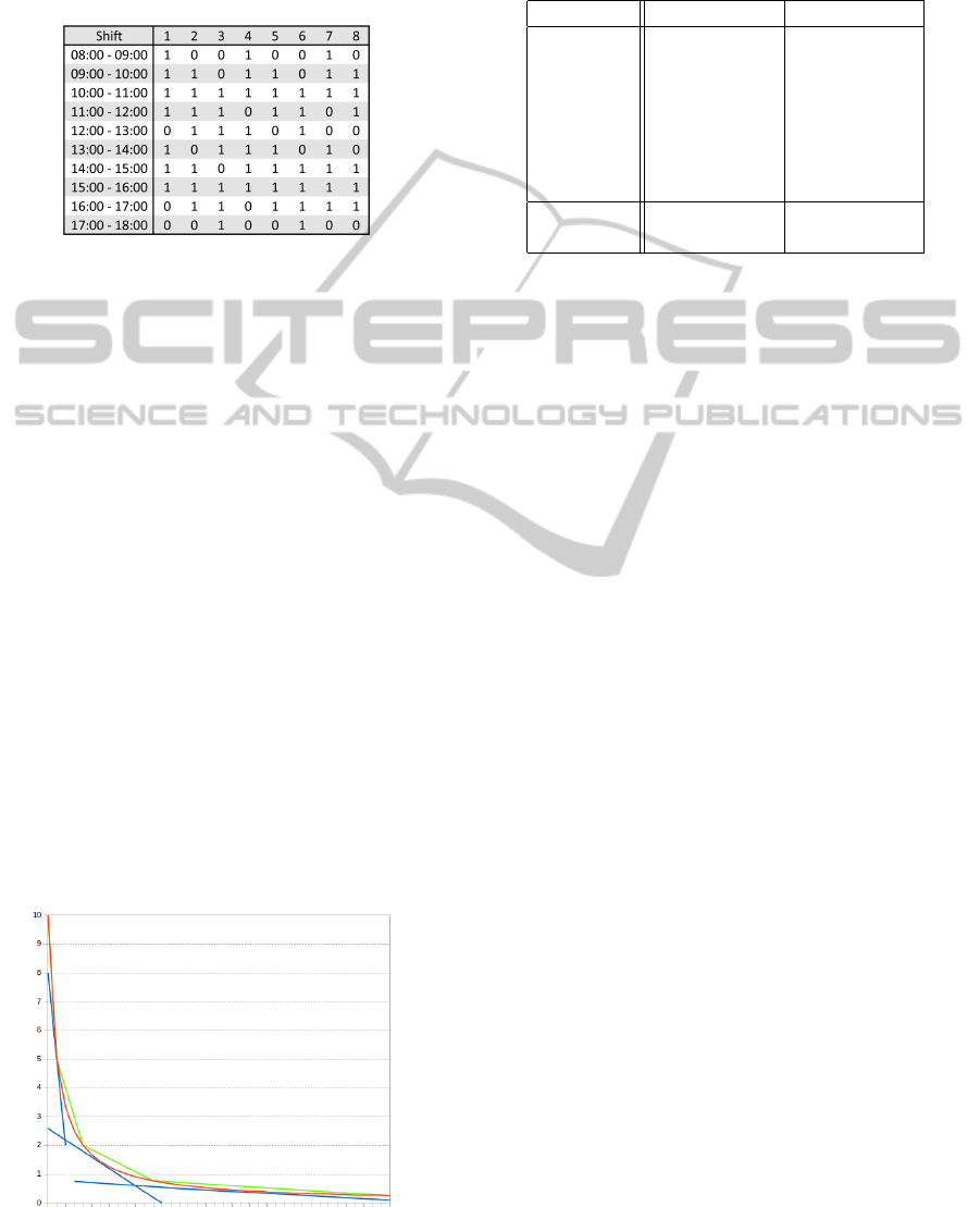
We consider here we want to schedule one day of 10
hours. We propose a simple matrix of 8 shifts with
1-hour periods.
Figure 1: Example of a simple shifts matrix.
For each period we consider a value of the call ar-
rival rate. For one day, let us consider the following
vector λ = {38; 77;82; 41; 18;53;75; 64; 54;29}. The
values of arrival rates for day follow a typical saison-
nality.
The queue parameters are the following: the goal
Average Speed of Answer ASA
∗
= 1 and the service
rate µ = 1.5.
Using the algorithm of Subsection 2.2, we are
able to compute the number of staff requirements:
b = {26; 52; 56;28; 13; 36;51;44; 37;20}.
For each period, let us consider values of vari-
ances: σ
2
= {1; 2;2; 1; 1;2;2; 2; 2;1}.
We then want to solve the distributionally robust
program (6). For this example, we set the risk level at
10%: ε = 0.10. Previous section gives us upper and
lower bounds of the problem. Then we consider the
two programs (13) and (16).
We choose several interpolation points y
j
. For
each period of time, there is one constraint for each
of the interpolation points.
Here is an illustration of the piecewise approxima-
tions of function f for :
Figure 2: Piecewise linear approximations of function f .
The solutions of the programs give the staffings
according to the possibles shifts. They are the given
in Table 1.
Table 1: Result for upper and lower bounds.
Shift Lower Bound Upper Bound
1 3 3
2 0 0
3 18 13
4 15 15
5 0 0
6 7 13
7 21 20
Total Staff 84 85
Cost 81.14 82
The Cost Gap here is CG = 0.011. Finally we can
compute Ax very easily if needed.
5 NUMERICAL EXPERIMENTS
5.1 Instance
In order to evaluate the quality and the robustness
of our model, we applied our approach to instances
based on data from a health insurance call center.
This data provides forecasts for one week from Mon-
day morning to Saturday midday (5 days of 10 hours
and 1 half-day of 3.5 hours). The horizon is split
in 30-minute periods. 24 differents shifts, from both
full-time and part-time schedules, make up the shifts
matrix. As we previously said in Section 2, we can
standardize the service rate µ without loss of general-
ity. We consider that all agents have the same hourly
salary, thus the cost of one agent is proportional to the
number of periods worked.
We computed the vectors of scheduled agents x
l
and x
u
for one week with the two programs (13)
and (16) of the previous section, providing an upper
bound and a lower bound of the optimal solution cost.
We used 17 points for computing the piecewise tan-
gent and linear approximations. We noticed that the
order of magnitude of variables y
t
is between 10
−2
and 10
−1
, thus we reduced the gap between the up-
per and lower bounds by gathering most of the points
around this area.
We want to evaluate the quality of our solutions
x
l
and x
u
. To this end we simulate possible realiza-
tions of arrival rates according to different distribu-
tions with the same data as previously. We consider
different possible distributions: gamma distributions,
uniform distribution, Pareto distribution, and varia-
ICORES2015-InternationalConferenceonOperationsResearchandEnterpriseSystems
10

Table 2: Results for different parameters.
Parameters Results
Variance range λ range ASA
∗
Risk ε Cost Gap % Violations
0.3 − 1 16 − 86 1 15% 0.0045 5 − 3
0.3 − 5 16 − 86 1 15% 0.011 1 − 0
0.1 − 1 4 − 20 1 15% 0.027 13 − 9
0.1 − 1 4 − 20 1 10% 0.034 7 − 4
2.5 − 9 4 − 20 0.3 15% 0.052 1 − 1
tions of normal distributions (log-normal, folded nor-
mal).
We elaborate a scenario as following: for each pe-
riod of time we simulate a call arrival rate according
to one of the given probability distributions. Then we
compute the number of effective required agents for
each period. A scenario covers requirements for the
whole time horizon. Finally we compare these val-
ues of requirements with our solutions of the problem
(lower solution x
l
and upper solution x
u
). A scenario
is considered as violated if at least in one period the
scheduled solution (by x
u
or x
l
is not enough in com-
parison of what the realization requires.
We computed between 100 and 500 scenarios for
each probability distributions. The percentage of vi-
olations gives us an idea of the robustness of our ap-
proach for several chosen distributions. The cost of
the solutions gives us an idea of the quality of the min-
imization.
5.2 Results
In Table 2, we give the percentage of violated scenar-
ios for various ranges of values of means and vari-
ances, and risk level. The queue parameters µ was set
to 1 as it simply represents a multiplicity factor. The
first column gives the range of values of the variances
through the day. The second column gives the range
of values of the means through the day, following a
typical seasonality.
The value Cost Gap (CG) of the 5th column is
given by the relative difference between the cost of
the upper bound solution and the cost of the lower
bound solution: CG =
c
t
x
u
−c
t
x
l
c
t
x
l
.
The last column gives the number of violated sce-
narios for the lower bound and for the upper bound.
In Table 2 we can notice that both upper and lower
bound solutions respect the set risk level. The varia-
tions of the parameters show that the bigger the vari-
ances, the better the model. The distributionally ro-
bust model deals very well with increasing of vari-
ances. We notice that even if we allow 15% risk, only
a few scenarios are violated when the variances are
higher (second and last lines of Table 2). In these
cases the call center is over-staffed and the given so-
lutions seem too conservative. But it is important to
remember that all the observations are based on simu-
lations of only a few examples of distributions. These
very low percentages only show that if the arrival rates
λs follow in reality one of the studied distributions, it
may be over-staffed. However the distributionally ro-
bust model indeed consists in taking all possible dis-
tributions with given mean and variance into account.
Thus it may be possible to reach the maximum risk
level with other particular distributions.
These results show that our approach is robust,
considering the numbers of violations never exceed
the risk level we set. The values of Cost Gap show
that the two bounds are close enough to propose a
very close solution to optimal solution.
We can notice that even if the solutions costs are
very close, the number of violations is different be-
tween the upper solution and the lower solution. This
is due to the fact that the distribution of the agents
through the different shifts is different according to
the programs.
Table 3 focuses on comparing results for different
risk levels. The simulations were made with these pa-
rameters:
• µ = 1
• λ follows a daily seasonality, varying between 4
calls/min and 21 calls/min
• σ
2
varies through the periods, between 0.25 and
1.
These parameters show well the performance of
the model. Table 3 gives the costs of the two bound
solutions and the Cost Gap. Like previously we ran
100 simulations and evaluated the number of violated
scenarios, which is given in the last column of the
table.
The first two columns of Table 3 gives the chosen
parameters. Columns 3 and 4 gives the solution costs
of the two programs and column 5 gives the Cost Gap.
Finally, the two last columns give the number of vio-
lated scenarios for the two solutions.
Unsurprisingly, the cost of the solution increases
when the risk level decreases. The Cost Gap seems
SchedulingProbleminCallCenterswithUncertainArrivalRatesForecasts-ADistributionallyRobustApproach
11
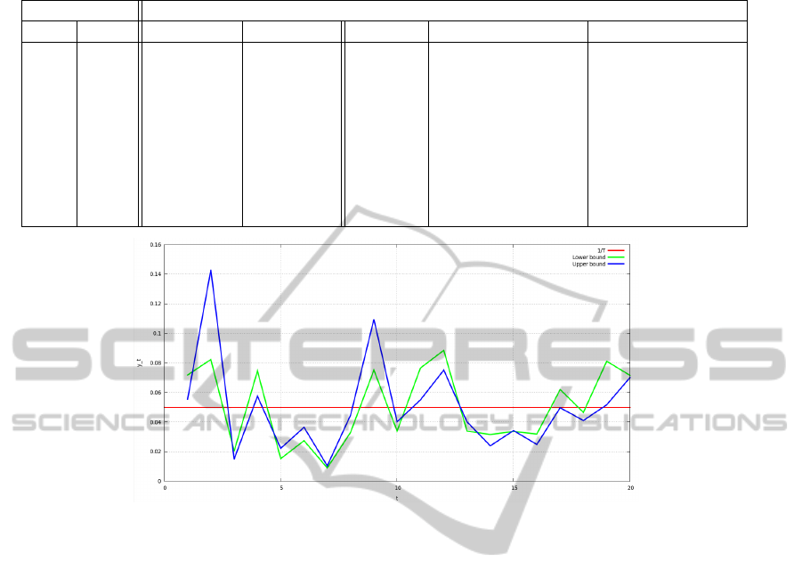
Table 3: Results for different risk levels.
Parameters Results
ASA
∗
Risk ε Lower Cost Upper Cost Cost Gap % Violations Upper % Violations Lower
5 15% 27 27.75 0.028 5 3
5 10% 29 30 0.034 2 1
5 05% 33.81 35.31 0.044 0 0
1 15% 27.5 28.5 0.036 7 4
1 10% 29.44 30.5 0.036 3 2
1 05% 34.31 35.88 0.046 1 1
0.3 15% 28.88 29.94 0.037 12 7
0.3 10% 31.12 32.19 0.034 5 2
0.3 05% 35.69 37.56 0.052 0 0
Figure 3: Sharing out of the risk through the day.
to remain in a small range, even if we notice a small
increase of the gap when the risk is lowered.
We can also see an increasing of the cost when
ASA
∗
(the objective Average Speed of Answer) de-
creases.
Like previously, the violations results show that
our model respects the initial risk conditions, for both
upper and lower solutions.
Figure 3 show the values of y
t
variables through
the horizon for the upper bound (in blue) and the
lower bound (in green). The red line shows the equal
division of the risk through the day. This figure brings
out the interest of dynamically sharing out the risk:
optimization of the variable y
t
shows their value are
different from the simple equal division through the
periods. Thus our approach is more complicated but
leads to cheaper solutions than a simpler approach
with fixed risk levels.
6 CONCLUSION
This paper presents a distributionally robust approach
for the staffing and shift-scheduling problem arising
in call center. We introduced the distributionally ro-
bust approach, considering that the call arrival rates
are following an unknown continuous distributions.
Moreover, instead of considering the risk level on a
period-by-period basis, we decided to set this risk
level for the whole horizon of study and thus consider
a joint chance-constrained program. Then, we pro-
posed a deterministic equivalent of the distribution-
ally robust approach with a dynamic sharing out of the
risk. We were thus able to propose solutions with re-
duced costs compared to other published approaches.
Finally we gave lower and upper bound of the prob-
lem with piecewise linear approximations. Compu-
tational results show that both upper and lower solu-
tions respect the objective risk level for a given set
of continuous distributions. This shows that our ap-
proach proposes robust solutions. The Cost Gap was
small enough to be able to bring out a valid solution
for the initial problem, which is eventually useful for
the managers.
In the simulations, we noticed that mainly the
Pareto distribution and Gamma distribution are the
ones with violated scenarios. The solutions of the
model show that for other distributions, the call cen-
ter may be over-staffed. Thus, we could study further
the call center model in order to evaluate what are the
interesting distributions to consider. This can lead, as
an improvment for our work in the future, to the study
ICORES2015-InternationalConferenceonOperationsResearchandEnterpriseSystems
12

of a given set of distributions, according to some con-
ditions (in addition to the known mean and variance).
Moreover, we can focus on improving the queuing
system model by considering another approach of the
representation of the service level in order to have a
closer representation to reality.
Another interesting future research would be to
conduct a sensitivity analysis that accounts for the
forecast bias.
Finally we made the assumption that periods of
the day are independent. In reality, we can notice a
daily correlation of the periods in a call center: busy
periods may appear in an entire busy day and rarely
alone. Conversely, light periods should lead to an en-
tire light day. We can then consider that the effective
arrival rates depend on a busyness factor, which rep-
resents this level of occupation of the day.
ACKNOWLEDGEMENTS
This research is funded by the French organism DIG-
ITEO.
REFERENCES
Aksin, Z., Armony, M., and Mehrotra, V. (2007). The mod-
ern call center: A multi-disciplinary perspective on
operations management research. Production and Op-
erations Management, 16:665–688.
Bertsimas, D. and Popescu, I. (1998). Optimal inequali-
ties in probability theory: A convex optimization ap-
proach. Technical report, Department of Mathematics
and Operations Research, Massachusetts Institute of
Technology, Cambridge, Massachusetts.
Brown, L., Gans, N., Mandelbaum, A., Sakov, A., Shen, H.,
Zeltyn, S., and Zhao, L. (2005). Statistical analysis of
a telephone call center: A queueing-science perspec-
tive. Journal of the American Statistical Association,
100:36–50.
Calafiore, G. C. and El Ghaoui, L. (2006). On distribution-
ally robust chance-constrained linear programs. Jour.
of Optimization Theory and Applications, 130:1–22.
Excoffier, M., Gicquel, C., Jouini, O., and Lisser, A. (2014).
Comparison of stochastic programming approaches
for staffing and scheduling call centers with uncertain
demand forecasts. In Communications in Computer
and Information Science, Lecture Notes in Computer
Science. Springer. To appear.
Gans, N., Koole, G., and Mandelbaum, A. (2003). Tele-
phone call centers: Tutorial, review, and research
prospects. Manufacturing & Service Operations Man-
agement, 5:79–141.
Gans, N., Shen, H., and Zhou, Y.-P. (2012). Parametric
stochastic programming models for call-center work-
force scheduling. Working paper.
Gross, D., Shortle, J. F., Thompson, J. M., and Harris, C. M.
(2008). Fundamentals of Queueing Theory. Wiley
Series.
Gurvich, I., Luedtke, J., and Tezcan, T. (2010). Staffing call
centers with uncertain demand forecasts: A chance-
constrained optimization approach. Management Sci-
ence, 56:1093–1115.
Liao, S., Koole, G., van Delft, C., and Jouini, O. (2012).
Staffing a call center with uncertain non-stationary ar-
rival rate and flexibility. OR Spectrum, 34:691–721.
Liao, S., van Delft, C., and Vial, J.-P. (2013). Distribu-
tionally robust workforce scheduling in call centers
with uncertain arrival rates. Optimization Methods
and Software, 28:501–522.
Luedtke, J., Ahmed, S., and Nemhauser, G. (2007). An in-
teger programming approach for linear programs with
probabilistic constraints. Integer Programming and
Combinatorial Optimization, 4513:410–423. Springer
Berlin Heidelberg.
Robbins, T. R. and Harrison, T. P. (2010). A stochastic
programming model for scheduling call centers with
global service level agreements. European Journal of
Operational Research, 207:1608–1619.
APPENDIX
Here we give the proof of the convexity of
f :]0; 1] → R
+
(17)
y 7→
r
p
y
1 − p
y
with p ∈ [0; 1[.
Function f is C
∞
, so we can compute the second
derivative of function f . We have first:
d f
dy
=
ln p
2
p
y
2
(1 − p
y
)
1
2
+
ln p
2
p
y
(1 − p
y
)
−
1
2
p
y
2
1 − p
y
=
ln(p)(1 − p
y
)
−
1
2
(p
y
2
(1 − p
y
) + p
3
2
y
)
2(1 − p
y
)
= f (y)
ln p
2(1 − p
y
)
Then,
d
2
f
dy
2
=
ln p
2
f
0
(y)(1 − p
y
) + ln(p)p
y
f (y)
(1 − p
y
)
2
=
ln
2
(p)(1 + 2p
y
)
4(1 − p
y
)
2
f (y)
=
ln
2
(p)(1 + 2p
y
)
4(1 − p
y
)
2
p
y
2
(1 − p)
y
2
(18)
Since every term of the second derivative is pos-
itive, we conclude that
d
2
f
dy
2
is positive and then, f is
convex.
SchedulingProbleminCallCenterswithUncertainArrivalRatesForecasts-ADistributionallyRobustApproach
13
