
Can We Find Deterministic Signatures in ECG and PCG Signals?
J. H. Oliveira
1
, V. Ferreira
2
and M. Coimbra
1
1
Instituto de Telecomunicações, Faculdade de Ciências da Universidade do Porto, Porto, Portugal
2
Faculdade de Ciências da Universidade do Porto, Porto, Portugal
Keywords: Deterministic Analysis, Heart Signal Processing, Predictability.
Abstract: The first step in any non linear time series analysis, is to characterize signals in terms of periodicity, station-
arity, linearity and predictability. In this work we aim to find if PCG (phonocardiogram) and ECG (electro-
cardiogram) time series are generated by a deterministic system and not from a random stochastic process.
If PCG and ECG are non-linear deterministic systems and they are not very contaminated with noise, data
should be confined to a finite dimensional manifold, which means there are structures hidden under the sig-
nal that could be used to increase our knowledge in forecasting future values of the time series. A non-linear
process can give rise to very complex dynamic behaviours, even though the underlying process is purely de-
terministic and probably low-dimensional. To test this hypothesis, we have generated 99 surrogates and then
we compared the fitting capability of AR (auto-regressive) models on the original and surrogate data. The
results show with a 99\% of confidence level that PCG and ECG were generated by a deterministic process.
We compared the fitting capability of an ECG and PCG to AR linear models, using a multi-channel ap-
proach. We make an assumption that if a signal is more linearly predictable than another one, it may adjust
better to these AR linear models. The results showed that ECG is more linearly predictable (for both chan-
nels) than PCG, although a filtering step is needed for the first channel. Finally we show that the false near-
est neighbour method is insufficient to identify the correct dimension of the attractor in the reconstructed
state space for both PCG and ECG signals.
1 INTRODUCTION
Over the last decades, there has been an increasing
interest in creating joint electrical-mechanical heart
models using multi-source signals from the cardiac
system. Therefore it seems crucial that we must
characterize these sources. Non-linear methods have
been successfully tested and used to study the
dynamics of the system. One interesting idea is that
aperiodicity in the data may not be due to a
stochastic process but due to a non-linear
deterministic system. False nearest neighbours
method (FNN) (Kaplan, 1992-1993) have been
widely and somewhat blindly used to estimate the
minimum necessary embedding dimension. (Hegger
and Kantz, 1999) identified some limitations on
FNN statistic in distinguishing between low-
dimensional chaotic data and their corresponding
surrogate data, giving as an example a simple ECG
record, although they did not make any assumptions
or claim that ECG signal is a deterministic process.
In this study, we have expanded Hegger's work
and incorporated PCG analysis in order to pave the
way for multi-source fusion of these signals into a
unified model. Possibly more importantly, we
performed a null-hypothesis experiment using
surrogate time series in order to distinguish and
quantify the differences between PCG and ECG
from a Gaussian stochastic process. This work's
primary aim is to study the deterministic behaviour
of a PCG and ECG signal. We aim to understand
which signal is more linearly predictable and as a
consequence more reliable. This will give us clues
on how to combine information from the acoustic
and electromagnetic system in order to create a more
interesting space capable of detecting pathological
diseases with higher accuracy than using a single
ECG or PCG approach. If the PCG and ECG are
deterministic signals then the secondary aim of this
paper is to estimate their embedding dimension. An
overestimation would lead to inaccurate results since
all coordinates would be contaminated by noise and
it also would lead to an increase in computational
effort as most of the operations for prediction or
classification scale exponentially with the
embedding dimension. Finally, it could also lead to a
184
H. Oliveira J., Ferreira V. and Coimbra M..
Can We Find Deterministic Signatures in ECG and PCG Signals?.
DOI: 10.5220/0005205201840189
In Proceedings of the International Conference on Bio-inspired Systems and Signal Processing (BIOSIGNALS-2015), pages 184-189
ISBN: 978-989-758-069-7
Copyright
c
2015 SCITEPRESS (Science and Technology Publications, Lda.)
poor performance of the general algorithm used,
simply because it treats the signal to be more
complicated than what it really is. A sub-estimation
would result in the incapacity of the system to
reconstruct the phase space.
This paper is structured as follows: ECG and
PCG morphologies are presented in section 2.
Surrogate time series are explained in section 3
followed by an introduction to false nearest
neighbours in section 4. Materials are presented in
section 5. Results and conclusions complete the
paper in sections 6 and 7.
2 ECG AND PCG
MORPHOLOGIES
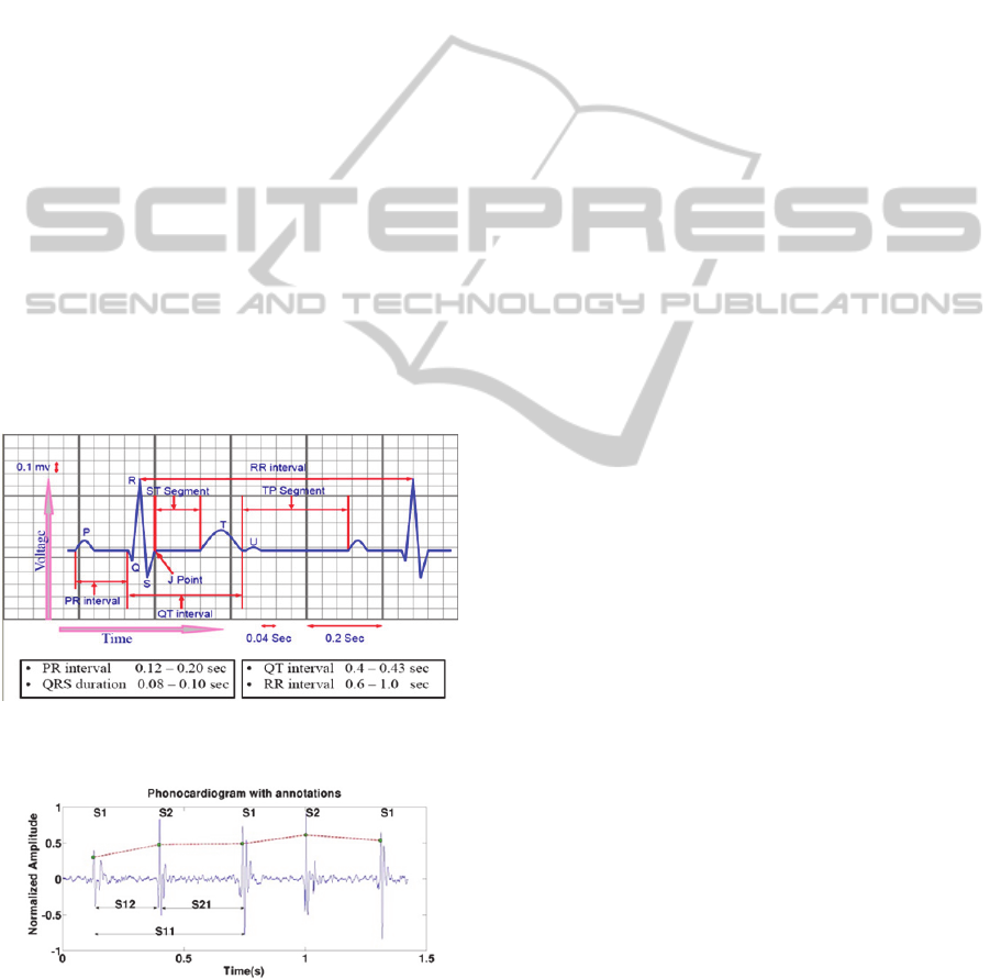
An electrocardiogram (ECG) is an electrical
signature of the heart and it can give us indicators of
pathological conditions. There are 3 main deflections
in an ECG (Figure 1): the P wave, QRS complex and
T-wave. These waves correspond to the far field
induced by specific electrical phenomena on the
cardiac surface, namely, the atrial depolarization P,
the ventricular depolarization, QRS complex, and
the ventricular repolarization T.
Figure 1: The main components and segments in an ECG
signal (adapted from (Guyton, 2006)).
Figure 2: A typical heart sound and its four main compo-
nents: S1, S2, Systole and Diastole.
In Figure 2 we can observe the various
components of a heart cycle, including S1 (first heart
sound) and S2 (second heart sound). These establish
the boundaries of the other two fundamental
components of a heart cycle: the systole (period
between S1 and S2), and the diastole (period
between S2 and S1). S1 and S2 are generated by the
opening and closing of the various heart valves and
in some auscultations we have the presence of
additional sounds such as S3, S4 or murmurs
(Guyton, 2006
)
.
3 SURROGATE TIME SERIES
The ECG and PCG signals gives us a time series. In
order to find a phase space we need to convert the
observations
into state vectors. A delay
reconstruction is formed by delay vectors given by :
,
,⋯,
1
(1)
Where n is the sample time, m is the embedding
dimension and is the delay time; the choice of the
two embedding parameters m andare crucial to
probe deterministic behaviour with minimal
computational effort. Taken's theorem (Kantz, 2004)
states that for ideal noise-free data, there exists a
dimension such that the delay vectors
are
equivalent to phase space vectors. If is enough for
this purpose every
will work as well, but
this redundancy when considering chaotic data leads
to a lower performance of many algorithms. In
particular, the noise that is always present
contaminates all the components of our delay vector
and the computational cost is higher, which
compromises any attempt for prediction or control.
Also in this way the minimum embedding dimension
gives us a lower bound on the dimensionality of the
system. The delay time measures the temporal
correlation between the states of
. If is small
compared to the time scales successive elements of
the delay vectors are strongly correlated. On the
other hand, for large successive elements are
almost independent. In the limit of infinite data and
infinite precision any time delay would work but in
reality we have a range of acceptable values for .
This motivates the search for optimal embedding
parameters
,
for our problem.
3.1 Algorithm to Generate the
Surrogates
In this paper the process to generate the surrogates
of the original data is the Iterated Amplitude
Adjusted Fourier Transform (IAAFT) surrogates,
since it already takes into account the bias towards a
CanWeFindDeterministicSignaturesinECGandPCGSignals?
185
too flat spectrum, when the length of the time series
is not large enough, like it happens in Amplitude
Adjusted Fourier Transform (AAFT) (Schreiber,
2000).
∣
∣
∣
∣
∣
∣
(2)
These components are multiplied by a random phase
where
are uniformly distributed in
0,2
and
. Different phases yield new surro-
gates. As a first step we apply a random shuffle to
that returns
. The i-th shuffle
must have the desired power spectrum.
This is accomplished taking the Fourier transform of
and replacing the squared amplitudes
,
by
and then transforming back.
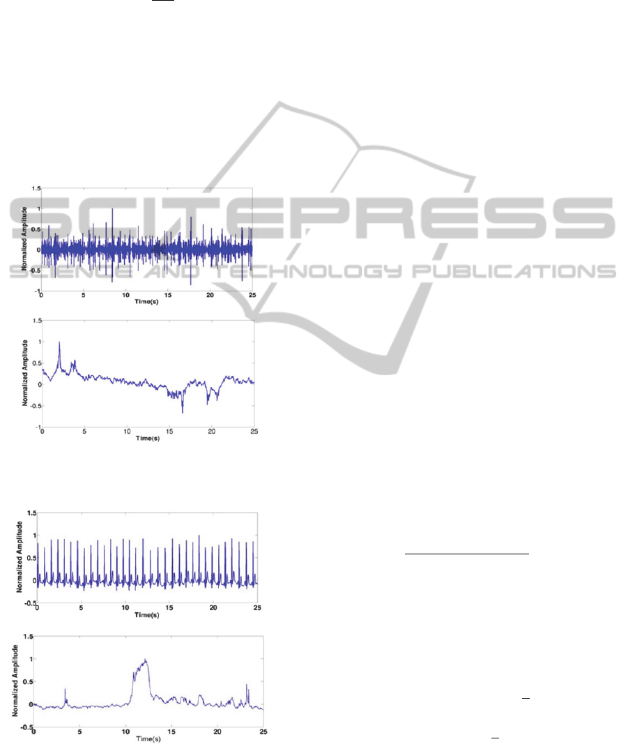
(3A)
(3B)
Figure 3: PCG signal (A) and it is corresponding surrogate
(B).
(4A)
(4B)
Figure 4: ECG signal (A) and it is corresponding surrogate
(B).
Although we achieve the correct spectrum, the dis-
tribution is modified. A second-step is required to
rank-order the resulting series to strictly assume the
values taken by
. This modifies the resulting
spectrum
so the 2 steps have to be repeated
several times until the algorithm converges. The
TISEAN implementation was used to this end
(Kantz, 2004).
3.2 The Null Hypothesis
The null hypothesis is defined for a time series in
terms of a class of processes that is assumed to
contain the specific process that generated the data
(Schreiber, 2000). In this section we are interested in
understanding the underlying dynamics of the signal,
mainly if deterministic signatures are present. In
other words, we want to test if the data was not
generated by a random stochastic process but by a
deterministic system. If that assumption is true, we
should observe temporal correlation in our data
points which is something that could not happen in a
surrogate time series, since any linear temporal
correlation between successive data points have
been completely destroyed by the process. We
choose the AR (autoregressive) linear model with
nonzero coefficients and two consecutive lag
samples.
1
2
(3)
Where
and
are the model coefficients. These
are calculated during the training phase using the
first half of the signal. After this optimization step,
the algorithm is going to predict the newest values
using the second half of the signal (equation (3)).
Finally the mean square error (̅
) is computed from
the observed and the predicted values, as it described
in equation (4).
̅
∑
(4)
We argue that if a signal is deterministic it may be
more predictable than a non-deterministic one,
unless in cases of very noisy systems. A pre-
processing step is thus recommended in order to
attenuate the noise. First we select a residual
probabilityof a false rejection, corresponding to a
level of significance
1
∗100%, then for the
one-sided test we generate
1 surrogate
sequences, whereis a positive integer
corresponding to a total of
sets. Therefore the
probability of the data has one of thesmallest
prediction errors is exactly. In our case, K is set
BIOSIGNALS2015-InternationalConferenceonBio-inspiredSystemsandSignalProcessing
186

equal to 1 in order to minimize the computational
effort, since mostly of the computational time is
generating the surrogates.
4 FALSE NEAREST NEIGH-
BOURS METHOD (FNN)
The False Nearest Neighbours (FNN) method was
developed (Kennel, 2002) to estimate the minimum
embedding dimension necessary to correctly
represent the dynamics of a system. It is based on
the uniqueness property of the phase space trajectory
for deterministic systems in which points that are
close in the phase space remain close under forward
interaction. The nearest neighbour of a point is
considered to be a false neighbour if they are close
purely by a projection effect. Therefore, the
optimized value for the embedding dimension is the
minimum value which correctly represents the
attractor (only for correlation dimension) (Kennel,
1992). For the implementation we take a
given
indimensions and find the nearest
neighbour
. The Euclidean distance in m-
dimensions is:
̃
(5)
The same is done for1dimensions, where this is
simply the previous vectors with an extra component
. So:
̃
(6)
The specific test for false neighbours is given as:
̃
(7)
If the increase in distance is larger than a given
threshold
(usually10
20) we name these
points as false nearest neighbours. When this
quantity drops to zero we have unfolded the attractor
into a m-dimensional Euclidean space.
4.1 FNN statistics
The previous criterion alone does not provide a safe
standard to determine a proper embedding
dimension. It is known that stochastic processes
(characterized by high dimensional attractors) yield
a vanishing or at least a small fraction of false
nearest neighbours. The fact is that even if
is
the closest neighbour to
when
is
comparable with the size of the attractor
the
criterion does not count this as a false neighbour. So,
a second test gives
as a false neighbour if :
̃
(8)
has typical values between 1 and 2.
is usually
chosen as :
1
̄
⁄
(9)
where ̄ is the average value of the observed data.
5 MATERIALS
The used dataset was collected in the Center for
Cardiothoracic Surgery (CCT-CHUC) and the
Cardiology Department (DCCHC-CHUC) of the
Centro Hospitalar e Universitário de Coimbra under
the scope of the HeartSafe project. The dataset is
composed by 33 healthy patients: 31 males and 2
females. The Body Mass Index average is 24 (BMI)
and their age average are 30 are summarized in
Table 1. Two ECG channels and one PCG were
recorded simultaneously and annotated by an expert
physician.
6 RESULTS
We test the null-hypothesis for both ECG and PCG
signals with and without filtering. The ECG signal is
filtered using a low-pass filter followed by high-pass
filter in order to form a bandpass filter in the 5-15Hz
frequency range and normalized at last. In Figure
3.A it is represented a typical phonocardiogram
signal (PCG), which was used to generate the surro-
gate data plotted in Figure 3.B. Different time lags
were chosen in order to demystify its importance in
the false nearest neighbours (FNN) statistic. The
results in Figure 5 showed a lack to sensitivity of the
false nearest neighbour method to distinguish the
original PCG from the surrogate. In other words,
both curves show the same trend regardless of the
dimensionality. These results can be extrapolated
easily to the ECG as it is shown in Figure 6 (Go-
vindan, 1998). The false nearest neighbour method
revealed itself as not capable to distinguish deter-
ministic from a stochastic process in both PCG and
ECG signals. All graphics plotted in Figures 5-6
show that the percentage of FNN tends to zero more
quickly for a higher embedding dimension , inde-
pendently of the time delay . This can be explained
CanWeFindDeterministicSignaturesinECGandPCGSignals?
187
by the fact of adding an extra
1
component
in a vector
of dimension. As an
alternative explanation, this can be due to a specific
geometric characteristic of the attractor. This topic
will be explored in future works. Regarding the
embedding dimension tested, the decay velocity is
faster in ECG than in PCG, which possibly means
that an ECG signal is more folded than a PCG one in
the reconstructed phase space. In some cases, it is
observable an increase in FNN statistics. This might
be happening because of noise, since a high dimen-
sion system is by nature more susceptible to it than a
lower one.
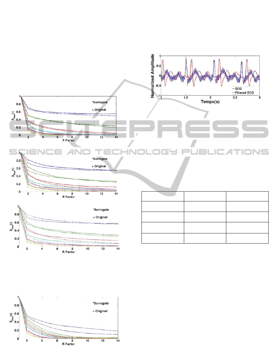
(A)1
(B)5
(C)10
Figure 5: Percentage of FNN for PCG data and their sur-
rogate for 1→6 (from top to bottom) using different
, R factor is the maximum distance between pairwise
points to be considered a true neighbours.
Figure 6: Percentage of FNN for ECG data and their sur-
rogate for 1→6 (from top to bottom) using 1, R
factor is the maximum distance between pairwise points to
be considered a true neighbours.
The null-hypothesis was designed to test if the ECG
and PCG data represents a deterministic process. In
order to create a 99% statistic significance test, we
have generated M = 99 surrogates using the IAAFT
algorithm. For the evaluation of the AR performance
in the surrogate data, we have followed the same
procedure discussed on the previous sections.
Figure 7: The ECG (blue) and its filtered (red) in channel
1. The bandpass filter used is adding a constant phase to
the original ECG signal.
We have tested the null-hypothesis using two ECG
and one PCG signal. The ECG signals were recorded
at 600Hz and 44100Hz sampling frequency from
two different channels (Figure 7). The PCG was
recorded at 44100Hz sampling frequency.
Table 2: Mean square error (̅
) from the Original ECG
and PCG series and their corresponding surrogates.
Ori
g
inal Surro
g
ate
Min
2.02E-3 1.70E-3
1.18E-7 7.65E-5
2.00E-7 8.43E-4
PCG 5.51E-6 1.47E-4
The HeartSafe dataset is composed by 960 seconds
of record in average, although we used records of
only 9.6 seconds to speed up the process. Results are
presented in Table 2.
With the exception of the non-filtered ECG in
channel 1, both PCG and ECG have smaller mean
square error (̅
) than their corresponding minimum
surrogate series. Therefore we can conclude with a
99% of confidence level that ECG and PCG were
not generated by a random stochastic system but
instead by a non-linear deterministic system. For the
non-filtered ECG in channel 1, the noise level was
unusually high (Figure 7), therefore the noisy
stochastic components are predominant under the
sources of information. This result lead to an
impossibility of rejecting the null-hypothesis for
such noisy levels.
BIOSIGNALS2015-InternationalConferenceonBio-inspiredSystemsandSignalProcessing
188

Table 3: HeartSafe dataset results.
ECG
Ch1
ECG
Ch2
PCG ECG Ch1
Filt
̅
3.29E-4 1.67E-7 1.87E-6 2.48E-7
We also compare the fitting capability of ECG and
PCG to AR linear models (Table 3). We make an
assumption that if a signal is more linearly
predictable than another one, it may adjust better to
these AR linear models. The HeartSafe dataset
results showed that filtered ECG is a more linearly
predictable signal than filtered PCG. The first ECG
channel exhibits higher noise levels when compared
to the second one, as a consequence ̅
is greater in
the first channel making it a more unreliable
channel.
7 CONCLUSIONS
Using a null hypothesis test, we concluded with 99%
of confidence that the PCG and ECG data came
from a deterministic system, although potentially
contaminated with a broad type of noises.
The FNN statistic revealed itself to be insufficient to
extract an embedding dimension from both PCG and
ECG signals, simply because it was never observed
a zero fraction of false neighbours. Therefore any
attempt to build a phase space turns to be
insufficient to completely describe the dynamical
system so the embedding dimension does not insure
a deterministic mapping. This can be caused by the
measurement noise (error which is independent of
the system, where all observations are contaminated
by some amount) or dynamical noise (feedback
process where in the system is perturbed by some
amount in each time step (Schreiber, 1996)).
Dynamical noise may sometimes be a higher
dimensional part of the dynamics with small
amplitude. At least one type of the dynamical noise
in a PCG is not static but it is periodic or quasi-
periodic and it depends on the breathing cycle,
making the analysis of PCG a more difficult task.
Finally, in the HeartSafe dataset, ECG revealed to be
a more linearly predictable signal when compared to
the PCG, although a filtering step is needed in
channel 1. Therefore, in order to improve the
predictability of a multi-signal acquisition system ,
we suggest to have more PCG than ECG channels,
since they are more linearly unpredictable signals.
ACKNOWLEDGEMENTS
This work was partially funded by the Fundação
para a Ciência e Tecnologia (FCT, Portuguese
Foundation for Science and Technology) under the
reference Heart Safe PTDC/EEI-PRO/2857/2012;
and Project I-CITY - ICT for Future
Health/Faculdade de Engenharia da Universidade do
Porto, NORTE-07-0124-FEDER-000068, Pest-
OE/EEI/LA0008/2013.
REFERENCES
D. T. Kaplan and L.Glass, Phys. Rev. Lett 68, 427 (1992).
D. T. Kaplan and L.Glass, Phys. Rev. Lett 64, 431 (1993).
T. Schreiber and A.Schmitz, Phys. Rev. Lett. 77. 635
(1996).
M. Kennel, H. Abarbanel, False neighbours and false
strands: A reliable minimum embedding dimension al-
gorithm, Phys. Rev.E, Vol 66, Nub 4, (2002).
A. Guyton, J.E.Hall, Textbook of Medical Physiology.
Elsevier Saunders, 11th ed, Ed Hall, (Jun 2006).
R. Hegger, H.Kantz, Improved false nearest neighbour
method to detect determinism in the time series data,
Phys. Rev. E, Vol 60, Numb 4, (Oct 1999).
T. Schreiber and A.Schmitz, Surrogate time series Physica
D, vol. 142, no 3-4, pp 34-382, (2000).
The TISEAN Software packet of Hegger, H. Kantz and T.
Schreiber can be download for free from :
http://www.mpipks-dresden.mpg.de/~tisean/
M. B. Kennel, R.Brown, and H.D.I Abarbanel, Phys. Rev.
A 45, 3403 (1992).
J. F. Kaiser, System Analysis by Digital Computer, chap. 7.
New York, Wiley (1996).
H. Kantz, T. Schreiber, Nonlinear Time Series Analysis ,
2th ed. Vol .3, Ed. Cambridge University Press, ( Jan
2004).
R. B. Govindan, K. Narayanan, and M. S. Gopinathan On
the evidence of deterministic chaos in ECG: Surrogate
and predictability analysis, Vol .8, Numb 2, Chaos
(June 1998).
CanWeFindDeterministicSignaturesinECGandPCGSignals?
189
