
Learning to Predict Video Saliency using Temporal Superpixels
Anurag Singh
1
, Chee-Hung Henry Chu
1,2
and Michael A. Pratt
3
1
Center for Advanced Computer Studies, University of Louisiana at Lafayette, Lafayette, LA, U.S.A.
2
Informatics Research Institute, University of Louisiana at Lafayette, Lafayette, LA, U.S.A.
3
W.H. Hall Department of Electrical and Computer Engineering,University of Louisiana at Lafayette, Lafayette, LA, U.S.A.
Keywords: Video Saliency, Temporal Superpixels, Support Vector Machines, Saliency Flow.
Abstract: Visual Saliency of a video sequence can be computed by combining spatial and temporal features that
attract a user’s attention to a group of pixels. We present a method that computes video saliency by
integrating these features: color dissimilarity, objectness measure, motion difference, and boundary score.
We use temporal clusters of pixels, or temporal superpixels, to simulate attention associated with a group of
moving pixels in a video sequence. The features are combined using weights learned by a linear support
vector machine in an online fashion. The temporal linkage for superpixels is then used to find the saliency
flow across the image frames. We experimentally demonstrate the efficacy of the proposed method and that
the method has better performance when compared to state-of-the-art methods.
1 INTRODUCTION
Finding what attracts a viewer’s attention in video
data has many applications in video analysis and
pattern recognition, such as video summarization,
video object recognition, surveillance, and
compression. In these applications, it is paramount
to find the salient object in the video. A majority of
work in predicting video saliency focuses on eye
tracking where the aim is to mimic human vision.
The major problem associated with eye-tracking
saliency maps is that they do not scale well with
higher level applications (Cheng et al., 2011), such
as object detection. In this paper we propose a new
method to detect salient objects in a video sequence
using feature integration theory.
Treisman and Gelade (1980) in their seminal
work described feature integration theory in which
visual attention is derived from many features in
parallel. These features are combined together
linearly to focus where the attention is at a salient
location. The weights in the combination step rank
the features according to their relative importance.
Building on this biological principle we propose
to use four features which attract attention in
parallel. These features are: (i) color contrast, which
is the most discriminant feature to differentiate a
salient vs non-salient region; (ii) motion difference,
which captures the change in the location of a salient
object; (iii) notion of objectness, which gives the
probability of occurrence of a generic object; and
(iv) boundary score, which is a measure of the
existence of boundary. In our method, the feature
combination step is achieved by learning the weights
using a linear support vector machine.
In a dynamic scene depicted in a video sequence,
the focus of attention tends to occur in clusters
(Mital et al., 2011) rather than at the pixel level.
Clustering of pixels into meaningful homogeneous
regions forms what are referred to as superpixels.
Temporal coherence between superpixels so that the
same superpixel belongs to same object across the
frames is accomplished by using temporal
superpixels (Chang et al., 2013).
The feature integration technique described
above finds the fixation in a single frame and in
principle we could just find attention separately for
every frame. Saliency detection for a single image
(frame) differs from that for video in that the viewer
has no continuous or prior information when
viewing a single image, so that there is no gaze
transition. In video saliency detection prior
information is essential to facilitate the gradual
transition of attention from one region of importance
to another over several frames. Transition from a
single frame to video is modeled by online learning
of weights and by using prior saliency information
from the previous frames to update the current frame
via a saliency flow framework.
201
Singh A., Henry Chu C. and A. Pratt M..
Learning to Predict Video Saliency using Temporal Superpixels.
DOI: 10.5220/0005206402010209
In Proceedings of the International Conference on Pattern Recognition Applications and Methods (ICPRAM-2015), pages 201-209
ISBN: 978-989-758-077-2
Copyright
c
2015 SCITEPRESS (Science and Technology Publications, Lda.)
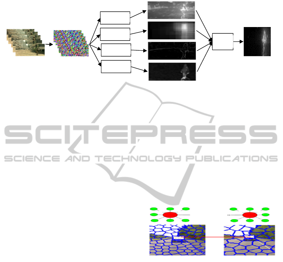
Figure 1: Flow diagram for detecting video saliency.
2 RELATED WORK
Itti and Baldi (2005) use the feature integration
theory to combine local cues of intensity, color,
orientation, motion in parallel using a center
surround map. A surprising change to a distribution
is captured by maximizing the posterior probability
of the combination map. Mahadevan and
Vasconcelos (2010) use a biologically inspired
discriminant center surround saliency hypothesis for
video where each pixel is represented by a spatio-
temporal patches which is contrasted with the center
to find saliency. Using rare or abnormal motion to
detect saliency in a video is proposed by Mancas et
al. (2011) where only dynamic features are used and
no static features such as color or contrast are
incorporated. Fukuchi et al. (2009) use a stochastic
representation of saliency map using Kalman filters.
Rudoy et al. (2013) present a method to predict
the gaze location given the previous frame fixation
map. They generate three sets of candidate maps as
static, semantic and motion maps. A random forest
classifier is trained to predict the location of the gaze
in the next frame. Our method extends their work in
that we use a learning-based feature integration
along with a Gaussian process-based superpixel
linkage (Chang et al., 2013) to generate video
saliency.
3 VIDEO SALIENCY
3.1 Temporal Superpixels
As fixation occurs in clusters it is useful to group
pixels together into regions. The so-called
superpixels are one way to do this grouping. Ren
and Malik (2003) use Gestalt principles for grouping
pixels into superpixels where a good grouping meant
that each group confirms to proximity, similarity and
homogeneity. Extension to video requires solving
that superpixel correspondence (Figure 2) that
entails ensuring a superpixel’s boundary remains
constant in subsequent frames under the constraints
of change in intensity, occlusion, camera movement
and deformation.
Figure 2: Temporal Superpixel Representation showing
superpixel correspondence.
There are existing methods for solving the
superpixel correspondence problem. Xu and Carso
(2012) provide an excellent review for supervoxels
based methods that extend superpixels to
supervoxels in video frames. A supervoxel can be
generated using the mean shift method (Paris and
Durand 2007), a graph based method (Grundmann et
al., 2010), segmentation by weighted aggregation
(Sharon et al., 2006), an energy optimization
framework (Veksler et al., 2010), or superpixels
rates for color histogram (Van den Bergh et al.,
2013). Supervoxels are over-segmented but not
regular sized so that the boundaries do not remain
the same.
Video
Temporal
superpixel
Salient
Features
SVM
Weights
Saliency
Flow
Final
map
Max
Peak
Frame 1 Frame N
Superpixel
correspondence
ICPRAM2015-InternationalConferenceonPatternRecognitionApplicationsandMethods
202
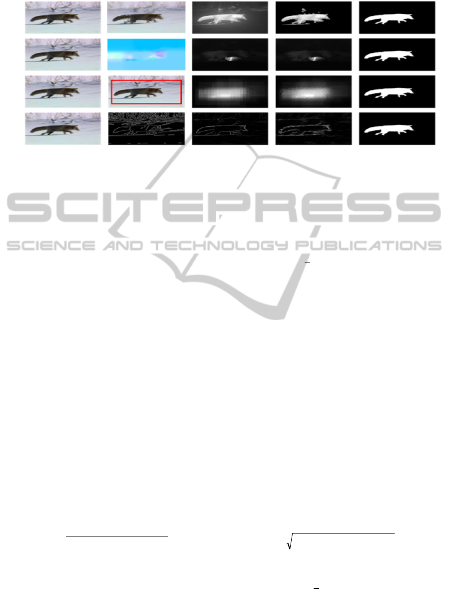
Figure 3: Feature Maps. Rows indicates features map associated with color, motion, objectness and boundary while column
shows input; intermediate level details (for color it is average color, for motion it is optical flow, for objectness it is
bounding box and for boundary it is edge map); pixel-level details; superpixel-level details; and ground truth.
To extend superpixels in its basic form for videos,
temporally consistent superpixels create a global
color space and superpixels are assigned to the color
space depending on an energy function and the
mutability of the sliding window frame (Reso et al.,
2013). In temporal superpixel, a temporally linked
superpixel is created in each frame by building a
generative graphical model using topological
constraints (Chang et al., 2013). We use temporal
superpixels as it gives regular shaped compact
superpixels with intact boundaries across frames.
3.2 Salient Features
Salient features are those which attract attention. In
our work, they are color dissimilarity, motion
difference, objectness, and boundary score. Figure 3
shows the feature maps computation at different
stages.
3.2.1 Color Dissimilarity
Color dissimilarity is measured by comparing the
color difference between superpixels. A group of
pixels is dissimilar with respect to other pixel groups
if it stands out (Goferman et al., 2010). The
dissimilarity for a pair of superpixels is given by
Singh et al. (2014) as
,
,
1
,
(1)
where
,
is the color difference
between superpixels computed as the distance
between two average colors in the CIE L*a*b* color
space and
,
is the position
difference between superpixel centers. The CIE
L*a*b* color space is used because it supports
chromatic double opponency. Further, we aggregate
the individual dissimilarities as follows,
1
,
(2)
where
is the global dissimilarity measure for
superpixel i, n is the number of superpixels and
,
is the local dissimilarity measure from
Equation 1. The global dissimilarity measure is
mapped to the saliency feature so that the higher the
global dissimilarity measure, the closer the saliency
is to 1. In our work, the color dissimilarity map is
given by color
i
= 1 – exp(–Gsp
i
).
3.2.2 Motion Difference
A change in motion attracts attention; to capture this
change we compute motion difference between
frames. At frame t, we first compute the optical flow
(Sun et al., 2010) to obtain at each pixel location the
horizontal and vertical velocity components denoted,
respectively,
),( yxu
t
and
),( yxv
t
. We compute the
changes in velocity components as
21
ttt
uuu
and
21
ttt
vvv
. The frame motion difference
is determined in terms of these changes:
22
),(),(),( yxvyxuyxf
ttt
.
(3)
The motion difference for superpixel r is given by
1
,
,
(4)
where J is the total number of pixels in the
Boundary Objectness Motion Color
LearningtoPredictVideoSaliencyusingTemporalSuperpixels
203
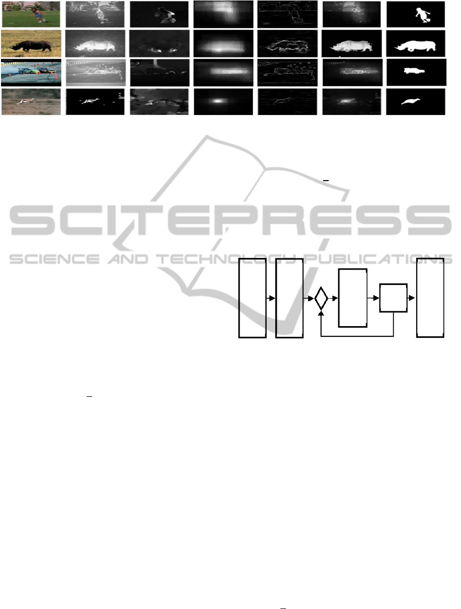
Figure 4: Individual features and integrated results (“Combined”) compared to Ground Truths.
superpixel and
,
are pixels in superpixel r at
frame . The motion difference ensures only fast
moving pixels which generate strong cues have a
stronger contribution towards saliency detection.
3.2.3 Objectness Measure
Human eyes are most tuned to be fixated on an
object in a scene. There can be one or many salient
objects in an image that can be anywhere in the
scene. The objectness map of an image is the
probability of occurrence of an object in a window
(Alexe et al., 2012). Sampling for object windows
gives the notion of objectness (Sun and Ling, 2013),
which ensures a higher probability value for the
occurrence of an object. Objectness for a superpixel
is computed by finding the average objectness of
underlying pixels in a superpixel as follows:
1
,
(5)
where
is the objectness for superpixel
r, J is the total pixels in superpixel r,
is the
probability of occurrence of an object in objectness
map (Sun and Ling 2013), and
,
is the location
of the jth pixel.
3.2.4 Boundary Score
Boundaries encompass both edges and corners in a
way that is more natural to human perception. Not
all edges attract attention but those pixels that do
attract attention often lie on a boundary. We
calculate a boundary score as a measure of how
likely a pixel is a boundary pixel. For boundary
detection we use the learned sparse code gradients
(Ren and Bo 2012). The boundary score of
superpixel r is given by
1
,
(6)
where J is the total pixels in superpixel r,
is
the boundary map of the image (Ren and Bo, 2012),
and
,
is the location of the jth pixel.
Figure 5: Online update of weights.
3.3 Feature Integration using SVM
The value of superpixel r in a saliency map, denoted
r
S
, is formed by a linear combination of the salient
features:
rbrm
rorcr
boundarywmotionw
objectnesswcolorwS
(7)
where the weights
,
,
,
are found by the
linear support vector machines (SVM) (Chang and
Lin, 2008). In the following, when we compute the
saliency value in a video sequence, we refer to the
saliency value for the
r
th superpixel in the
th
frame as
,r
S
.
A linear SVM when given a training set
,
,
∈
,
∈
1,1
,1,…,, solves
the following unconstrained problem:
min
,
1
2
,;
,
(8)
Input Color Motion Objectness Boundary Combined Ground Truth
Features
Wei
g
hts
New Wei
g
hts
ICPRAM2015-InternationalConferenceonPatternRecognitionApplicationsandMethods
204
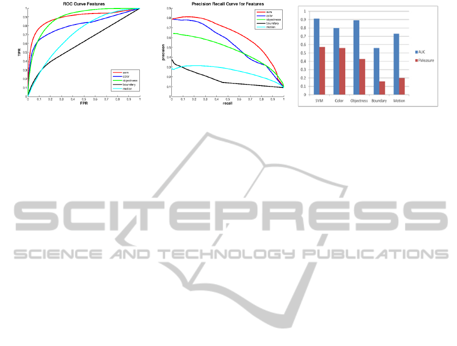
Figure 6: Combination map generated using feature integration (labeled “svm”) gives better performance over individual
maps.
where is the weight vector,
,
are, respectively,
the data and label of instance i, is the penalty
parameter, and ,;
,
is the loss function.
These weights give the importance of each feature
and they can be viewed as activation functions
which enhance certain features and inhibit others.
Figure 4 shows the feature integration results.
Learning and updating the weights at each frame
using online gradient descent (Karampatziakis and
Langford, 2010) is as follows
(9)
where
is the weight vector for next frame,
is
the weight for the current frame and
is the
loss function. Here the data
is the combination
map and
is the ground truth. Figure 5 shows the
process of updating weights.
3.4 Saliency Flow
Video is rich in redundancy in the context of
saliency information. Human gaze lasts nearly 5 to
10 frames before shifting in a video (Koffka, 1955).
Inter-frame saliency dependence is strong so that a
salient superpixel in a current frame is most likely to
be salient in the previous frame. This gives us a
chain like structure between superpixels (“old
superpixels”) that exists in a previous frame. An old
superpixel may change its size due to perspective
change but its boundary remains the same. If a
superpixel pops up in the current frame it is called a
“new superpixel.”
There are many centers of activation in an image
which can influence saliency. We extend it to video
by finding the center of activation in T previous
frames; in our work, we set
5T
corresponding to
the lower end of the human gaze duration. For an old
superpixel, the activation center is found by finding
the most salient superpixel in
T
previous frames.
For a new superpixel we find the closest nearest
neighbor which can influence its saliency. A
superpixel feature is given by the feature vector
〈
̅,,
,,,
〉
consisting of the average location,
CIE L*a*b* color channel values, and texture
information. This feature vector is used for a nearest
neighbor search. Figure 7b shows a pictorial
reference to this search process. Temporal
superpixels give the temporal linkage from which
we find the center of activation from a set of
previous frames that has the maximum influence on
the current superpixel r:
NewSPrS
OldSPrS
mv
ktr
Tk
ktr
Tk
r
,
,,1
,
,,1
ˆ
max
max
(10)
where
,
is the saliency from Equation 7 for the
same superpixel in frame
,
,
∈
is the value from
Equation 7 for the closest superpixel in frame
,
=
t–1,…, t–T. The current frame’s saliency for
superpixl r is updated from the previous frames by
2
⁄
(11)
where
is activation center’s saliency value
found for superpixel
and
is the saliency value
for the current superpixel
.
4 EXPERIMENTS
Algorithm 1 shows the steps for computing saliency
map. Training was done using 10-fold cross valida-
tion which resulted in an accuracy of 92.7%. The
importance of features found using SVM weight
vector is in the following order: objectness, color
dissimilarity, boundary score, and motion difference.
We test our algorithm on the Segtrack and Fukuchi
data sets. Segtrack (Tsai et al., 2012) is widely used
a: ROC curve. b: Precision Recall curve. c: Area under curve (AUC) and F-Measure.
LearningtoPredictVideoSaliencyusingTemporalSuperpixels
205
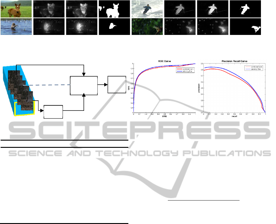
Figure 7a: Saliency Flow improves results over individual frames. “GT” refers to ground truth.
Figure 7b: Search for activation center (Saliency Flow). Figure 7c: ROC curve Figure 7d: Precision Recall Curve.
Algorithm 1: Video Saliency Detection
1. Compute temporal superpixels for each frame
a. for each superpixel do
1) Compute color dissimilarity Eq. 2;
2) Compute motion difference Eq. 4;
3) Compute objectness Eq. 5;
4) Compute boundary score Eq. 6;
2. Learn weights using linear SVM
a. update weights using online gradient decent
b. Generate combination map using learned
weights Eq. 7;
3. Compute saliency flow to account for temporal
consistency Eq. 10 ;
4. Generate final map.
for figure-ground segmentation and tracking. It has
16 videos with a total of 976 frames with one or
more objects along with such characteristics as
motion blur, appearance change, complex
deformation, occlusion, slow motion and interacting
objects. The Fukuchi et al. (2009) dataset has 10
natural scenes videos consisting of 936 frames with
one object.
We perform quantitative evaluations to show (i)
that feature combination maps out performs
individual features, (ii) that saliency flow generates
a better saliency map than single frame maps, and
(iii) that our method outperforms other state-of-the-
art methods.
Evaluation metrics are consistent for all three sets
of experiment. We use the benchmark code by Borji
et al. (2012) to ensure standard evaluations results.
We compute the area under the ROC curve. This
area shows how well the saliency algorithm predicts
against the ground truth. Precision is defined as the
ratio of salient object to ground truth, so that the
higher the precision the more the saliency map
overlaps with the ground truth. The recall measure
quantifies the amount of ground truth detected. The
weighted harmonic mean measure or F-Measure
(Cheng et al., 2011) of precision and recall is given
as
1
∙∙
∙
(12)
where
is set at 0.3. The data set used for
evaluation is a combination of the Segtrack and
Fukuchi data sets. We also perform qualitatively
evaluation using example images.
Feature Combination Evaluation:
We compute
four feature maps and the final integrated map learnt
using SVM weights. Figure 6a shows the average
ROC curve; Figure 6b shows precision-recall curve;
Figure 6c shows the area under curve and the F-
Measure. From these plots, we can see that the
integrated map out-performs all other feature maps.
Saliency Flow Evaluation:
The ROC curve in
Figure 7c and the precision-recall curve in Figure 7d
as well as the visual comparison in Figure 7a show
that saliency flow improves saliency detection.
Comparison to State-of-the-art Methods:
In order
to compare our work we use ROC curve (Figure 8a),
precision-recall curve (Figure 8b) and visual
comparison (Figure 9) with other saliency detection
methods (Table 1).
Input Single Frame Saliency Flow GT Input Single Frame Saliency Flow GT
Old
Activation
center
NN
New
Final
map
ICPRAM2015-InternationalConferenceonPatternRecognitionApplicationsandMethods
206
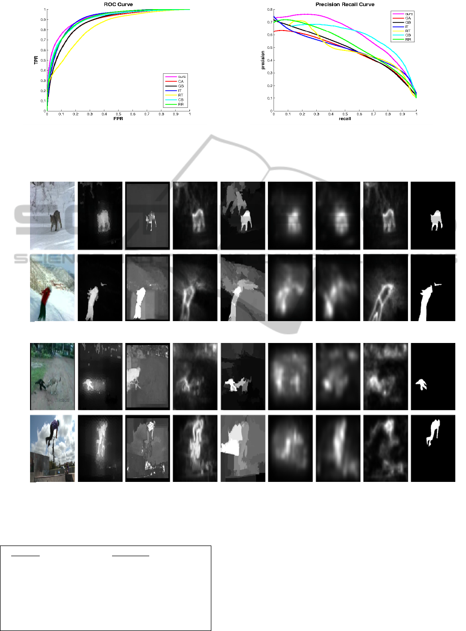
Figure 8: Comparisons of our method (“ours”) with other state of art methods (see Table 1) using the ROC and the
Precision Recall curves.
Figure 9: Visual comparisons of our results (“ours”) with other state-of-the-art methods. See Table 1 for method references.
Table 1: Saliency detection methods for comparison.
Method
Reference
IT (Itti and Baldi, 2005)
RR (Mancas et al., 2011)
JP (Fukuchi et al., 2009)
RT (Rahtu et al., 2010)
CA (Goferman et al., 2010)
CB (Jiang et al., 2011)
GB (Harel et al., 2007)
Methods IT, RR, JP and RT are video saliency
algorithms while CA, CB are among the best
methods that find salient objects (Borji et al., 2012);
GB has the best performance among eye-tracking
methods. We use the authors’ implementations to
generate video saliency map for the Fukuchi and
Segtrack data sets. From the comparison result we
can quantitatively establish that our methods out-
perform other methods.
a: ROC curve. b: Precision Recall curve.
Fukuchi Dataset
Input Ours RT CA CB GB IT JP GT
Segtrack Dataset
Input Ours RT CA CB GB IT RR GT
LearningtoPredictVideoSaliencyusingTemporalSuperpixels
207

5 CONCLUSIONS
We proposed a video saliency detection method
based on using SVM to learn weights for combining
features represented by superpixel clusters. The
process of combining features in the new algorithm
performs better than any individual feature. The
saliency flow from a video sequence generates a
better saliency map than single frame maps. We
compared our new method to other state-of-the-art
methods using publically available data sets and
showed that the new method has better performance.
The reported result is the first known application of
temporal superpixels for video saliency detection.
Our ongoing work is in visual tracking, in which we
find the most salient object along with temporal
linkage. The saliency map with salient objects can
also be used to guide video segmentation.
ACKNOWLEDGMENTS
The authors thank the reviewers whose suggestions
improved the manuscript. This work was supported
in part by the Louisiana Board of Regents through
grant no. LEQSF (2011-14)-RD-A-28.
REFERENCES
Alexe, B., Deselaers, T., and Ferrari, V., 2012. Measuring
the objectness of image windows. IEEE Transactions
on PAMI, vol. 34, no. 11, pp. 2189-2202.
Borji, A., Sihite, D.N., and Itti, L., 2012. Salient object
detection: A benchmark. In ECCV, pp. 414-429.
Chang, J., Wei, D., and Fisher, J.W., 2013. A video
representation using temporal superpixels. In IEEE
CVPR, pp. 2051-2058.
Chang Y., and Lin, C.-J., 2008. Feature ranking using
linear SVM. JMLR Workshop and Conference
Proceedings, vol. 3, pp. 53-64.
Cheng, M.-M., Zhang, G.-X., Mitra, N.J., Huang, X., and
Hu, S.-M., 2011. Global contrast based salient region
detection. In IEEE CVPR, pp.409-416.
Fukuchi, K., Miyazato, K., Kimura, A., Takagi S., and
Yamato, J., 2009. Saliency-based video segmentation
with graph cuts and sequentially updated priors.
In ICME, pp.638-641.
Goferman, S., Zelnik-Manor, L., and Tal, A., 2010.
Context-aware saliency detection. In IEEE CVPR, pp.
2376-2383.
Grundmann, M., Kwatra, V., Han, M. and Essa, I., 2010.
Efficient hierarchical graph-based video segmentation.
In IEEE CVPR, pp. 2141-2148.
Harel, J., Koch, C., and Perona, P., 2007. Graph-Based
Visual Saliency. In NIPS, pp. 545-552.
Itti L., and Baldi, P. 2005. A principled approach to
detecting surprising events in video. In IEEE CVPR,
pp. 631-637.
Jiang, H., Wang, J., Yuan, Z., Liu, T., Zheng, N., and Li.
S., 2011. Automatic salient object segmentation based
on context and shape prior. In BMVC, pp 7
Karampatziakis, N., and Langford, J. 2010. Online
importance weight aware updates. In UAI, pp 392-399.
Koffka, K., 1955. Principles of Gestalt Psychology.
Routledge & Kegan Paul.
Mahadevan, V., and Vasconcelos, N., 2010. Spatio-
temporal saliency in dynamic scenes. IEEE
Transactions on PAMI, vol. 32, no. 1, pp. 171-177.
Mancas, M., Riche, N., Leroy, J., and Gosselin, B., 2011.
Abnormal motion selection in crowds using bottom-up
saliency. In IEEE ICIP, pp. 229-232.
Mital, P.K., Smith, T.J., Hill, R.L., and Henderson, J.M.,
2011. Clustering of gaze during dynamic scene
viewing is predicted by motion. Cognitive
Computation, vol. 3, no. 1, pp. 5-24.
Paris S., and Durand, F., 2007. A topological approach to
hierarchical segmentation using mean shift. In IEEE
CVPR, pp. 1-8.
Rahtu, E,. Kannala, J., Salo, M., and Heikkilä, J., 2010.
Segmenting salient objects from images and videos. In
ECCV,
pp. 366-379.
Ren, X., and Bo, L., 2012. Discriminatively trained sparse
code gradients for contour detection. In NIPS, pp. 584-
592.
Ren, X., and Malik, J., 2003. Learning a classification
model for segmentation. In IEEE ICCV, pp. 10-17.
Reso, M., Jachalsky, J., Rosenhahn, B., and Ostermann, J.,
2013. Temporally consistent superpixels. In IEEE
ICCV, pp. 385-392.
Rudoy, D., Goldman, D.B., Shechtman, E., and Zelnik-
Manor, L., 2013. Learning video saliency from human
gaze using candidate selection. In IEEE CVPR, pp.
1147-1154.
Sharon, E., Galun, M., Sharon, D., Basri, R., and Brandt,
A., 2006. Hierarchy and adaptivity in segmenting
visual scenes. Nature, vol. 442, no. 7104, pp.719-846.
Singh, A., Chu, C.H., Pratt, M.A., 2014. Multiresolution
superpixels for visual saliency detection. In IEEE
Symposium on Computational Intelligence for
Multimedia, Signal, and Vision Processing.
Sun, J., and Ling, H., 2013. Scale and object aware image
thumbnailing. International Journal of Computer
Vision, vol. 104, no. 2, pp. 135-153.
Sun, D., Roth, S., and Black, M.J., 2010. Secrets of optical
flow estimation and their principles. In IEEE CVPR,
pp. 2432-2439.
Treisman, A.M., and Gelade. G., 1980. A feature-
integration theory of attention. Cognitive Psychology,
vol 12, no. 1, pp 97-136.
Tsai, D., Flagg, M., Nakazawa, A., and Rehg, J.M., 2012.
Motion coherent tracking using multi-label MRF
optimization. International Journal of Computer
Vision vol. 100, no.2, pp. 190-202.
ICPRAM2015-InternationalConferenceonPatternRecognitionApplicationsandMethods
208

Van den Bergh, M., Roig, G., Boix, X., Manen, S., and
Van Gool, L., 2013. Online video seeds for temporal
window objectness. In IEEE ICCV, pp. 377-384.
Veksler, O., Boykov, Y., and Mehrani, P., 2010.
Superpixels and supervoxels In an energy optimization
framework. In ECCV, pp. 211-224.
Xu, C., and Corso, J.J., 2012. Evaluation of super-voxel
methods for early video processing. In IEEE CVPR,
pp. 1202-1209.
LearningtoPredictVideoSaliencyusingTemporalSuperpixels
209
