Alignment of Cyclically Ordered Trees

∗

Takuya Yoshino

and Kouichi Hirata

Graduate School of Computer Science and Systems Engineering, Kyushu Institute of Technology,

Kawazu 680-4, Iizuka 820-8502, Japan

Department of Artiﬁcial Intelligence, Kyushu Institute of Technology, Kawazu 680-4, Iizuka 820-8502, Japan

Keywords:

Alignment, Alignment Distance, Segmental Alignment Distance, Cyclically Ordered Tree, Tai Mapping.

Abstract:

In this paper, as unordered trees preserving the adjacency among siblings, we introduce the following three

kinds of a cyclically ordered tree, that is, a biordered tree that allows both a left-to-right and a right-to-left order

among siblings, a cyclic-ordered tree that allows cyclic order among siblings in a left-to-right direction and a

cyclic-biordered tree that allows cyclic order among siblings in both left-to-right and right-to-left directions.

Then, we design the algorithms to compute the alignment distance and the segmental alignment distance

between biordered trees in O(n

) time and ones between cyclic-ordered trees and cyclic-biordered trees in

O(n

) time, where n is the maximum number of nodes and D is the maximum degree in two given trees.

1 INTRODUCTION

Comparing tree-structured data is one of the impor-

tant tasks for many research areas such as pattern

recognition, natural language processing, machine

learning, data mining, bioinformatics, and so on. In

these researches, the tree-structured data are well re-

garded as rooted labeled trees (trees, for short). Also

a tree is ordered if the left-to-right order among sib-

lings is ﬁxed and unordered otherwise.

An edit distance (Tai, 1979) is one of the standard

distance measures between trees. The edit distance is

formulated as the minimum cost to transform from a

tree to another tree by applying edit operations of a

substitution, a deletion and an insertion to trees.

It is known that the edit distance is closely related

to a Tai mapping (Tai, 1979). The minimum cost of

Tai mappings coincides with the edit distance (Tai,

1979). Then, whereas the problem of computing the

edit distance between ordered trees is tractable (De-

maine et al., 2009), one between unordered trees

is MAX SNP-hard (Zhang and Jiang, 1994). This

MAX SNP-hardness holds even if both trees are bi-

nary (Hirata et al., 2011).

An alignment distance is an alternative distance

measure between trees introduced by (Jiang et al.,

∗

This work is partially supported by Grant-in-Aid

for Scientiﬁc Research 24240021, 24300060, 25540137,

26280085 and 26370281 from the Ministry of Education,

Culture, Sports, Science and Technology, Japan.

1995) and applied to comparing RNA secondary

structures in bioinformatics (H¨ochsmann et al., 2003;

Schiermer and Giegerich, 2013; Shapiro and Zhang,

1990; Zhang, 1998). The alignment distance is for-

mulated as the minimum cost of possible alignments

(as trees) obtained by ﬁrst inserting nodes labeled

with spaces into two trees such that the resulting trees

have the same structure and then overlaying them. In

operational, the alignment distance is an edit distance

such that every insertion precedes to deletions.

Kuboyama (Kuboyama, 2007) has ﬁrst formulated

an alignable mapping as a variation of the Tai map-

ping. Then, he has shown that the alignment dis-

tance coincides with the minimum cost of alignable

mappings and the alignable mapping coincides with a

less-constrained mapping (Lu et al., 2001). As same

as the edit distance, whereas the problem of comput-

ing the alignment distance between ordered trees is

tractable, one between unordered trees is MAX SNP-

hard (Jiang et al., 1995). On the other hand, this prob-

lem becomes tractable if the degrees of unordered

trees are bounded (Jiang et al., 1995).

In the above results of computing distances, we

deal with either ordered or unordered trees. Note

that unordered trees allow all of the permutations

among siblings. On the other hand, several appli-

cations require to allow just some permutations, not

all of the permutations, among siblings. For exam-

ple, when representing graphs with cyclic compounds

such as monosaccharides in glycans (Hizukuri et al.,

263

Yoshino T. and Hirata K..

Alignment of Cyclically Ordered Trees.

DOI: 10.5220/0005207802630270

In Proceedings of the International Conference on Pattern Recognition Applications and Methods (ICPRAM-2015), pages 263-270

ISBN: 978-989-758-076-5

 2015 SCITEPRESS (Science and Technology Publications, Lda.)

2005) and molecules in molecular graphs (Horv´ath

et al., 2010) as trees, the adjacency of nodes in the

compounds is represented as the adjacency among

siblings in the tree representation. Also, when

comparing or modeling RNA secondary structures

as trees (H¨ochsmann et al., 2003; Schiermer and

Giegerich, 2013; Shapiro and Zhang, 1990; Zhang,

1998), the base pairs in nucleotides are connected

with preserving the adjacency among siblings.

Hence, as unordered trees preserving the adja-

cency among siblings, in this paper, we formulate

the following three kinds of a cyclically ordered

tree. Let v

, . .. , v

be siblings from left to right.

Then, we say that a tree is biordered if it allows

two orders v

, . . . , v

and v

, . . . , v

. Also we say

that a tree is cyclic-ordered if it allows a cyclic

order v

, . . . , v

, v

, . . . , v

i−1

for every i (1 ≤ i ≤ n).

Furthermore, we say that a tree is cyclic-biordered

if it allows cyclic orders v

, . . . , v

, v

, . . . , v

i−1

and

, . . . , v

, v

, . . . , v

i−1

for every i (1 ≤ i ≤ n).

Since an unordered binary tree is always cycli-

cally ordered, the problem of computing the edit dis-

tance, the segmental distance (Kan et al., 2014) and

the bottom-up distance (Valiente, 2001; Kuboyama,

2007) between cyclically ordered trees is also

MAX SNP-hard (Hirata et al., 2011; Yamamoto

et al., 2014). On the other hand, the problems of

computing the isolated-subtree (or constrained) dis-

tance (Zhang, 1995; Zhang, 1996), the accordant

(or Lu’s) distance (Lu, 1979; Kuboyama, 2007),

the LCA-preserving (or degree-2) distance (Zhang

et al., 1996) and the top-down (or degree-1) dis-

tance (Selkow, 1977; Chawathe, 1999) between un-

ordered trees are tractable, so are the problems of

computing these distances between cyclically ordered

trees.

In this paper, we focus on the alignment dis-

tance and a segmental alignment distance, which is

an alignment distance to preserve the parent-children

relationship as possible (Yoshino and Hirata, 2013),

between cyclically ordered trees, because the prob-

lems of computing both distances are tractable if the

degrees of unordered trees are bounded. Note that the

algorithms to compute all of the above tractable vari-

ations of the edit distance between unordered trees

contain the maximum weighted bipartite matching al-

gorithm (Yamamoto et al., 2014; Zhang et al., 1996)

or originally the minimum cost maximum ﬂow algo-

rithm (Wang et al., 2003; Zhang, 1996).

On the other hand, in this paper, by directly ex-

tending the recurrences to compute the alignment dis-

tance between ordered trees (Jiang et al., 1995), we

ﬁrst design the algorithms to compute the alignment

distance between biordered trees in O(n

) time,

where n is the maximum number of nodes and D is the

maximum degree in two given trees. This time com-

plexity is same as one between ordered trees (Jiang

et al., 1995). Also we design the algorithms to com-

pute the alignment distance between cyclic-ordered

and cyclic-biordered trees in O(n

) time.

Next, by using the same strategy of (Kan et al.,

2014) to compute a top-down distance for every pair

of nodes in given two cyclically ordered trees in ad-

vance, we design the algorithm to compute the seg-

mental alignment distance between cyclically ordered

trees with the same time complexity as above.

Finally, we give experimental results for the

alignment distance between biordered trees com-

paring with the edit distance between ordered

trees, by using N-glycan data provided from

KEGG (Kyoto Encyclopedia of Genes and Genomes,

http://www.kegg.jp/

2 PRELIMINARIES

A tree is a connected graph without cycles. For a tree

T = (V, E), we denote V and E by V(T) and E(T),

respectively. Also the size of T is |V| and denoted by

|T|. We sometime denote v ∈ V(T) by v ∈ T. We

denote an empty tree by

A rooted tree is a tree with one node r chosen as

its root. We denote the root of a rooted tree T by

r(T). For each node v in a rooted tree with the root

r, let UP

(v) be the unique path from v to r. The

parent of v(6= r), which we denote by par(v), is its

adjacent node on UP

(v) and the ancestors of v(6= r)

are the nodes on UP

(v) − {v}. We denote the set of

all ancestors of v by anc(v). We say that u is a child

of v if v is the parent of u. The set of children of v is

denoted by ch(v). We call the number of children of

v the degree of v and denote it by d(v), that is, d(v) =

|ch(v)|. Also we deﬁne d(T) = max{d(v) | v ∈ T}

and call it the degree of T.

In this paper, we use the ancestor orders < and ≤,

that is, u < v if v is an ancestor of u and u ≤ v if u < v

or u = v. We say that w is the least common ancestor

of u and v, denoted by u⊔ v, if u ≤ w, v ≤ w and there

exists no w

′

such that w

′

≤ w, u ≤ w

′

and v ≤ w

′

. A

(complete) subtree of T = (V, E) rooted by v, denoted

by T[v], is a tree T

′

= (V

′

, E

′

) such that r(T

′

) = v,

′

= { u ∈ V | u ≤ v} and E

′

= { (u, w) ∈ E | u, w ∈ V

′

We say that a rooted tree is labeled if each node

is assigned a symbol from a ﬁxed ﬁnite alphabet Σ.

For a node v, we denote the label of v by l(v), and

sometimes identify v with l(v). Also let ε 6∈ Σ denote

a special blank symbol and deﬁne Σ

= Σ∪ {ε}.

We say that a rooted tree is ordered if a left-to-

ICPRAM2015-InternationalConferenceonPatternRecognitionApplicationsandMethods

264

right order among siblings is ﬁxed; unordered oth-

erwise. In particular, for nodes u and v in an or-

dered tree, u is to the left of v, denoted by u  v,

if pre(u) ≤ pre(v) and post(u) ≤ post(v) for the pre-

order number pre and the postorder number post.

Furthermore, in this paper, we introduce cyclically

ordered trees by using the following functions σ

p,n

(i)

and σ

−

p,n

(i) for 1 ≤ i, p ≤ n.

p,n

(i) = ((i+ p− 1) mod n) + 1,

−

p,n

(i) = ((n− i− p+ 1) mod n) + 1.

Deﬁnition 1 (Cyclically Ordered Trees). Let T be a

tree and suppose that v

, . . . , v

are the children of v ∈

T from left to right.

1. We say that T is biordered if T allows the orders

of both v

, . . . , v

and v

, . . . , v

2. We say that T is cyclic-ordered if T allows the

orders v

p,n

(1)

, . . . , v

p,n

(n)

for every 1 ≤ p ≤ n.

3. We say that T is cyclic-biordered if T allows the

orders v

p,n

(1)

, . . . , v

p,n

(n)

and v

−

p,n

(1)

, . . . , v

−

p,n

(n)

for every 1 ≤ p ≤ n.

Sometimes we use the scripts o, b, c, cb, u, and the no-

tation of π ∈ {o, b, c, cb, u} , which we call a π-tree.

It is obvious that the cyclically ordered trees are

an extension of ordered trees and a restriction of un-

ordered trees. The number of orders among siblings

of a node v in ordered trees, biordered trees, cyclic-

ordered trees, cyclic-biordered trees and unordered

trees is 1, 2, d(v), 2d(v) and d(v)!, respectively.

Next, we introduce the alignment distance (Jiang

et al., 1995). Here, for π ∈ {o, b, c, cb, u}, we call an

isomorphism for π-trees a π-isomorphism.

Deﬁnition 2 (Alignment (Jiang et al., 1995)). Let T

and T

be trees and π ∈ {o, b, c, cb, u}. An alignment

between T

and T

is a tree T obtained by the follow-

ing two steps.

1. Insert new nodes labeled by ε into T

and T

such

that the resulting trees T

′

and T

′

are π-isomorphic

with ignoring labels and l(φ(v)) 6= ε whenever

l(v) = ε for a π-isomorphism φ between T

′

and

′

and every node v ∈ T

′

2. Set T to an obtained tree T

′

by relabeling a la-

bel l(v) for every node v ∈ T

′

with (l(v), l(φ(v))).

(Note that (ε, ε) 6∈ T .)

Let A

, T

) denote the set of all possible align-

ments between T

and T

We deﬁne a cost function γ : (Σ

×Σ

−{(ε, ε)}) 7→

on pairs of labels. We constrain γ to be a metric,

that is, γ(l

, l

) ≥ 0, γ(l

, l

) = 0, γ(l

, l

) = γ(l

, l

)

and γ(l

, l

) ≤ γ(l

, l

) + γ(l

, l

). In particular, we

sometimes use a unit cost function such that γ(l

, l

) =

1 if l

6= l

. The cost of an alignment T , denoted by

γ(T ), is the sum of the costs of all labels in T .

Deﬁnition 3 (Alignment Distance (Jiang et al.,

1995)). Let π ∈ {o, b, c, cb, u}. Then, the alignment

distance between T

and T

is deﬁned as the mini-

mum cost γ(T ) for every alignment T ∈ A

, T

Also we call an alignment with the minimum cost an

optimal alignment.

Example 1. Consider ordered trees T

and T

in Fig-

ure 1 (left). Then, T in Figure 1 (right) is the opti-

mal alignment between T

and T

. Under the unit cost

function γ, since γ(T ) = 4, the alignment distance be-

tween T

and T

is 4.

Figure 1: Ordered trees T

and T

(left) and the optimal

alignment T ∈ A

, T

) (right) in Example 1.

3 MAPPING AND DISTANCE

In this section, we introduce a Tai mapping and its

variations, and then the distance as the minimum cost

of all the mappings.

Deﬁnition 4 (Tai Mapping (Tai, 1979)). Let T

and

be trees and M ⊆ V(T

) ×V(T

1. We say that a triple (M, T

, T

) is an ordered

Tai mapping from T

to T

, denoted by M ∈

TAI

, T

), if every pair (u

, v

) and (u

, v

) in

M satisﬁes the following conditions.

(i) u

= u

iff v

= v

(one-to-one condition).

(ii) u

≤ u

iff v

≤ v

(ancestor condition).

(iii) u

 u

iff v

 v

(sibling condition).

2. We say that a triple (M, T

, T

) is an unordered

Tai mapping from T

to T

, denoted by M ∈

TAI

, T

), if M satisﬁes the conditions (i) and

(ii).

In the following, let u

, u

∈ ch(u) and

, v

∈ ch(v).

3. We say that a triple (M, T

, T

) is a biordered

Tai mapping from T

to T

, denoted by M ∈

TAI

, T

), if M satisﬁes the above conditions

(i) and (ii) and the following condition (iv).

(iv) For every u ∈ T

and v ∈ T

such that

, v

), (u

, v

), (u

, v

) ∈ M, one of the fol-

lowing statements holds.

1. u

 u

iff v

 v

AlignmentofCyclicallyOrderedTrees

265

2. u

 u

iff v

 v

4. We say that a triple (M, T

, T

) is a cyclic-ordered

Tai mapping from T

to T

, denoted by M ∈

TAI

, T

), if M satisﬁes the above conditions

(i) and (ii) and the following condition (v).

(v) For every u ∈ T

and v ∈ T

such that

, v

), (u

, v

), (u

, v

) ∈ M, one of the fol-

lowing statements holds.

1. u

 u

iff v

 v

2. u

 u

iff v

 v

3. u

 u

iff v

 v

5. We say that a triple (M, T

, T

) is a cyclic-

biordered Tai mapping from T

to T

, denoted by

M ∈ M

TAI

, T

), if M satisﬁes the above condi-

tions (i) and (ii) and the following condition (vi).

(vi) For every u ∈ T

and v ∈ T

such that

, v

), (u

, v

), (u

, v

), (u

, v

) ∈ M, one of

the following statements holds.

1. u

 u

iff v

 v

2. u

 u

iff v

 v

3. u

 u

iff v

 v

4. u

 u

iff v

 v

5. u

 u

iff v

 v

6. u

 u

iff v

 v

7. u

 u

iff v

 v

8. u

 u

iff v

 v

We will use M instead of (M, T

, T

) simply.

Since a less-constrained mapping (Lu et al., 2001)

coincides with an alignable mapping (Kuboyama,

2007) characterizing the alignment, we formulate the

alignable mapping as the less-constrained mapping.

Deﬁnition 5 (Variations of Tai Mapping). Let T

and

be trees, π ∈ {o, b, c, cb, u} and M ∈ M

TAI

, T

Here, we denote M− {(r(T

), r(T

))} by M

−

1. We say that M is an alignable map-

ping (Kuboyama, 2007) (or a less-constrained

mapping (Lu et al., 2001)), denoted by

M ∈ M

ALN

, T

), if M satisﬁes the follow-

ing condition.

∀(u

, v

), (u

, v

), (u

, v

) ∈ M



⊔ u

< u

⊔ u

=⇒ v

⊔ v

= v

⊔ v



2. We say that M is a segmental mapping (Kan et al.,

2014), denoted by M ∈ M

, T

), if M satisﬁes

the following condition.

∀(u, v) ∈ M

−



∃(u

′

, v

′

) ∈ M



′

∈ anc(u)) ∧ (v

′

∈ anc(v))



=⇒



(par(u), par(v)) ∈ M





3. We say that M is a segmental alignable map-

ping (Yoshino and Hirata, 2013), denoted by

M ∈ M

SGALN

, T

), if M ∈ M

, T

) ∩

ALN

, T

4. We say that M is a top-down mapping (Selkow,

1977; Chawathe, 1999) (or a degree-1 mapping),

denoted by M ∈ M

TOP

, T

), if M satisﬁes the

following condition.

∀(u, v) ∈ M

−



(par(u), par(v)) ∈ M



Let M be a mapping from T

to T

. Let I and J be

the sets of nodes in T

and T

but not in M. Then, the

cost γ(M) of M is given as follows.

γ(M) =

∑

(u,v)∈M

γ(u, v) +

∑

u∈I

γ(u, ε)+

∑

v∈J

γ(ε, v).

Deﬁnition 6 (Variations of Edit Distance). For every

A ∈ {TAI, ALN, SGALN, TOP} and π ∈ { o, b, c, cb, u},

we deﬁne the distance τ

, T

) as follows.

, T

) = min{γ(M) | M ∈ M

, T

)}.

Theorem 1. Let T

and T

be trees and π ∈

{o, b, c, cb, u}.

1. τ

TAI

, T

) coincides with the edit distance (Tai,

1979).

2. τ

ALN

, T

) coincides with the alignment dis-

tance (Kuboyama, 2007).

Theorem 2. Let T

and T

be trees such that n =

| ≥ |T

| = m and D = max{d(T

), d(T

)}.

1. We can compute τ

TAI

, T

) in O(nm

(1 +

log

)) = O(n

) time. On the other hand, the

problem of computing τ

TAI

, T

) is MAX SNP-

hard, even if T

and T

are binary (Demaine

et al., 2009; Zhang and Jiang, 1994; Hirata et al.,

2011).

2. We can compute τ

ALN

, T

) and τ

SGALN

, T

)

in O(nmD

) time. On the other hand, the prob-

lem of computing τ

ALN

, T

) and τ

SGALN

, T

)

is MAX SNP-hard, but it is tractable if the de-

grees of T

and T

are bounded (Jiang et al., 1995;

Yoshino and Hirata, 2013).

Proposition 1 (cf. (Kuboyama, 2007; Yoshino and

Hirata, 2013)). Let T

and T

be trees and π ∈

{o, b, c, cb, u}. Also suppose that a cost function is

a metric. Then, τ

TAI

, T

) and τ

TOP

, T

) are met-

rics, whereas neither τ

ALN

, T

) nor τ

SGALN

, T

)

is a metric.

Proposition 2. Let T

and T

be trees. For A ∈

{TAI, ALN, SGALN, TOP} and π ∈ {o, b, c, cb, u} , the

following statements hold.

1. τ

, T

) ≤ τ

, T

) ≤ τ

, T

) ≤ τ

, T

2. τ

, T

) ≤ τ

, T

) ≤ τ

, T

) ≤ τ

, T

ICPRAM2015-InternationalConferenceonPatternRecognitionApplicationsandMethods

266

3. τ

TAI

, T

) ≤ τ

ALN

, T

) ≤ τ

SGALN

, T

) ≤

TOP

, T

Proposition 3. For A ∈ {TAI, ALN, SGALN, TOP},

there exist trees T

and T

satisfying each of the fol-

lowing conditions.

1. τ

, T

) < τ

, T

2. τ

, T

) < τ

, T

Proof. Consider the following trees T

, T

and T

Under the unit cost function, Statement 1 follows

that τ

TOP

, T

) = 1 < 3 = τ

TOP

, T

) and Statement

2 followsthat τ

TOP

, T

) = 1 < 3 = τ

TOP

, T

Proposition 4. Let T

and T

be trees and A ∈

{TAI, ALN, SGALN, TOP}.

1. If max{d(T

), d(T

)} ≤ 1, then it holds

that τ

, T

) = τ

, T

) = τ

, T

) =

, T

) = τ

, T

2. If max{d(T

), d(T

)} ≤ 2, then it holds that

, T

) = τ

, T

) = τ

, T

) = τ

, T

3. If max{d(T

), d(T

)} ≤ 3, then it holds that

, T

) = τ

, T

Proposition 5. For π ∈ {b, c, cb}, there exist trees T

and T

satisfying each of the following conditions.

1. τ

TAI

, T

) < τ

ALN

, T

2. τ

ALN

, T

) < τ

TAI

, T

Proof. Consider the following trees T

, T

and T

and

suppose that a cost function is the unit cost function.

1. It is obvious that τ

TAI

, T

) = 2. On the other

hand, since the alignment T

is an optimal alignment

between T

and T

for cyclically ordered trees, it holds

that τ

ALN

, T

) = τ

ALN

, T

) = τ

ALN

, T

) = 3.

Note that τ

ALN

, T

) = 4 (Jiang et al., 1995).

2. Since the alignment T

is an optimal

alignment between T

and T

for cyclically ordered

trees, it holds that τ

ALN

, T

) = τ

ALN

, T

) =

ALN

, T

) = 1. On the other hand, it is obvious that

TAI

, T

) = 4. Note that τ

ALN

, T

) = 5.

4 ALGORITHMS

In this section, we identify a node with its pos-

torder number. Also let n = |T

|, m = |T

| (and sup-

pose that n ≥ m), d = min{d(T

), d(T

)} and D =

max{d(T

), d(T

)}.

A(n ordered) forest is a sequence [T

, . . . , T

] of

trees. For a tree T and a node i ∈ T, T(i) is a

forest obtained by deleting the root i in T[i]. For

nodes i ∈ T

and j ∈ T

, let the children of i and

j be i

, . . . , i

and j

, . . . , j

. That is, it holds that

d(i) = s and d( j) = t. Also, for trees T

and T

we denote the forests T

(i) = [T

], . . . , T

]] and

( j) = [T

[ j

], . . . , T

[ j

]] by F

, i

) and F

( j

, j

For A ∈ {ALN, SGALN, TOP} andπ ∈ {o, b, c, cb},

the recurrences in Figure 2 compute the distance τ

and the forest distance δ

when containing an empty

tree or forest. Also Figure 3 illustrates the common

recurrences Γ

and ∆

to compute τ

and δ

(

0) = 0,

[i],

0) = δ

(i),

0) + γ(i, ε),

(

0, T

[ j]) = δ

(

0, T

( j)) + γ(ε, j),

(i),

0) =

∑

k=1

0),

(

0, T

( j)) =

∑

k=1

(

0, T

[ j

]).

Figure 2: The basic recurrences of computing τ

, T

[i], T

[ j])

= min







[i],

0) + min

T∈T

(i)

{τ

(T, T

[ j]) − τ

(T,

0)},

(

0, T

[ j]) + min

T∈T

( j)

{τ

[i], T) − τ

(

0, T)}







∆

, i

), F

( j

, j

))

= min







, i

s−1

), F

( j

, j

)) + τ

0),

, i

), F

( j

, j

t−1

)) + τ

(

0, T

[ j

]),

, i

s−1

), F

( j

, j

t−1

)) + τ

], T

[ j

])







Figure 3: The common recurrences Γ

, T

) and

∆

, F

Let T

(i) = [T

], . . . , T

]] and T

( j) =

[ j

], . . . , T

[ j

]]. Also let 1 ≤ p ≤ s and 1 ≤ q ≤ t.

Then, we denote the forests [T

p,s

(1)

], . . . , T

p,s

(s)

]]

and [T

[ j

q,t

(1)

], . . . , T

[ j

q,t

(t)

]] by T

(i) and T

( j).

Also we denote the forests [T

−

p,s

(1)

], . . . , T

−

p,s

(s)

]]

and [T

[ j

−

q,t

(1)

], . . . , T

[ j

−

q,t

(t)

]] by T

−p

(i) and T

−q

( j).

It is obvious that T

(i) = T

(i) and T

( j) = T

( j).

AlignmentofCyclicallyOrderedTrees

267

Furthermore, the values of p and q in T

(i),

), T

( j) and T

( j

) are (1) p = q = 1 if π = o,

(2) p = ±1 and q = ±1 if π = b, (3) 1 ≤ p ≤ s and

1 ≤ q ≤ t if π = c and (4) 1 ≤ p ≤ s, −s ≤ p ≤ −1,

1 ≤ q ≤ t and −t ≤ q ≤ −1 if π = cb. Hence, we

prepare the following sets: (1) o(s) = o(t) = {1} , (2)

b(s) = b(t) = {−1, 1}, (3) c(s) = {1, . . . , s}, c(t) =

{1, . . . ,t}, and (4) cb(s) = {−s, . . . , −1, 1, . . . , s},

cb(t) = {−t, . . . , −1, 1, . . .,t}. We refer these sets to

π(s) and π(t) for π ∈ {o, b, c, cb}.

Then, by introducing the sets π(s) and π(t) into

the recurrences in (Jiang et al., 1995), we design the

recurrences of computing τ

ALN

, T

) between cycli-

cally ordered trees T

and T

as Figure 4.

ALN

[i], T

[ j])

= min

(

min

p∈π(s),q∈π(t)

{δ

ALN

(i), T

( j)) + γ(i, j)},

ALN

[i], T

[ j])

)

ALN

, i

), F

( j

, j

)) = min











∆

ALN

, i

), F

( j

, j

)),

γ(i

, ε)

+ min

1≤k<t,p∈π(s)



ALN

, i

s−1

), F

( j

, j

k−1

))

+δ

ALN

), F

( j

, j

)))



γ(ε, j

)

+ min

1≤k<s,q∈π(t)



ALN

, i

k−1

), F

( j

, j

t−1

))

+δ

ALN

, i

), T

( j

)))













Figure 4: The recurrences of computing τ

ALN

, T

) be-

tween cyclically ordered trees.

Theorem 3. The recurrences in Figure 4 are correct

to compute τ

ALN

, T

) between cyclically ordered

trees T

and T

for π ∈ {b, c, cb}.

Proof. In the proof of (Jiang et al., 1995) showing

that the recurrences of computing τ

ALN

, T

) is cor-

rect, the formulas and the cases of an optimal align-

ment tree or forest T are presented as follows.

1. The formula δ

ALN

(i), T

( j)) + γ(i, j) is corre-

sponding to the case that (i, j) is a label in an op-

timal alignment tree T of T

[i] and T

[ j], and T

contains the alignment of T

(i) and T

( j).

2. The formula

γ(i

, ε) + min

1≤k<t



ALN

, i

s−1

), F

( j

, j

k−1

))

+δ

ALN

), F

( j

, j

)))



is corresponding to the case that (i

, ε) is a label

in an optimal alignment forest T of F

, i

) and

( j

, j

), and T contains the alignment of T

)

and F

( j

, j

) for 1 ≤ k < t.

3. The formula

γ(ε, j

) + min

1≤k<s



ALN

, i

k−1

), F

( j

, j

t−1

))

+δ

ALN

, i

), T

( j

)))



is corresponding to the case that (ε, j

) is a la-

bel in an optimal alignment forest T of F

, i

)

and F

( j

, j

), and T contains the alignment of

, i

) and T

( j

) for 1 ≤ k < s.

In just above three formulas, an optimal alignment

T contains and expands the siblings of some node in

or T

(or both). When extending from τ

ALN

, T

)

to τ

ALN

, T

), it is sufﬁcient to deal with more than

two orders in the above three formulas, instead of one

left-to-right order, and then to replace T

(i), T

( j),

) and T

( j

) with T

(i), T

( j), T

) and T

( j

)

for p ∈ π(s) and q ∈ π(t). Hence, by replacing the for-

mulas in the above statements 1, 2 and 3 with the ﬁrst

formula in τ

ALN

, i

), F

( j

, j

)) and the second

and the third formulas in δ

ALN

, i

), F

( j

, j

)) in

Figure 4, we can compute τ

ALN

, T

) correctly.

Theorem 4. We can compute τ

ALN

, T

) in

O(nmD

) time. Also we can compute τ

ALN

, T

) and

ALN

, T

) in O(nmdD

) time.

Proof. In Figure 4, the number of recurrences in τ

ALN

is 3 and one in δ

ALN

is 5; the number of recurrences

in τ

ALN

is 6 and one in δ

ALN

is 7; the number of re-

currences in τ

ALN

is d(i)d( j) + 2 and one in δ

ALN

d(i) + d( j) + 3; the number of recurrences in τ

ALN

4d(i)d( j) + 2 and one in δ

ALN

is 2d(i) + 2d( j) + 3.

According to the proof of (Jiang et al., 1995),

for s = d(i) and t = d( j), we can compute

ALN

′

, i

), F

( j

′

, j

)) in O((s − s

′

) × (t − t

′

) ×

((s− s

′

) + (t −t

′

))) = O(d(i)d( j)(d(i) + d( j))) time.

Then, we can compute δ

ALN

′

, i

), F

( j

′

, j

)) in

O(d(i)d( j)(d(i) + d( j))) time. So the running time

of computing τ

ALN

[i], T

[ j]) for each (i, j) ∈ T

is O(d(i)d( j)(d(i) + d( j))d(i) + d(i)d( j)(d(i) +

d( j))d( j)) = O(d(i)d( j)(d(i) + d( j))

). Hence, the

running time of computing τ

ALN

, T

) is:

∑

i=1

∑

j=1



d(i)d( j)(d(i) + d( j))



≤

∑

i=1

∑

j=1



d(i)d( j)(d(T

) + d(T

))



≤ O



(d(T

) + d(T

))

∑

i=1

d(i) ×

∑

j=1

d( j)



≤ O(|T

| × |T

| × (d(T

) + d(T

))

)

= O(nmD

Also, by focusing on the number of recurrences in

Figure 4, we can compute δ

ALN

′

, i

), F

( j

′

, j

))

and δ

ALN

′

, i

), F

( j

′

, j

)) in O((s −

′

)d( j) × (t − t

′

)d(i) × ((s − s

′

) + (t − t

′

))) =

O(d(i)

d( j)

(d(i) + d( j))) time. So the run-

ning time of computing τ

ALN

[i], T

[ j]) and

ALN

[i], T

[ j]) for each (i, j) ∈ T

× T

ICPRAM2015-InternationalConferenceonPatternRecognitionApplicationsandMethods

268

O(d(i)

d( j)

(d(i) + d( j))d(i) + d(i)

d( j)

(d(i) +

d( j))d( j)+d(i)d( j)) = O(d(i)

d( j)

(d(i)+d( j))

where the last formula d(i)d( j) is corresponding to

the time complexity of computing the ﬁrst recurrence

in τ

ALN

[i], T

[ j]) in Figure 4. Hence, the running

time of computing τ

ALN

, T

) and τ

ALN

, T

) is:

∑

i=1

∑

j=1



d(i)

d( j)

(d(i) + d( j))



≤

∑

i=1

∑

j=1



d(i)d( j)d(T

)d(T

)

×(d(T

) + d(T

)



≤ O







d(T

)d(T

)(d(T

) + d(T

))

∑

i=1

d(i) ×

∑

j=1

d( j)







≤ O(|T

| × |T

| × d(T

)d(T

)(d(T

) + d(T

))

)

= O(nmdD

Next, we design the algorithm to compute the

segmental alignment distance τ

SGALN

, T

) for π ∈

{b, c, cb}. Here, we adopt the same strategy of (Kan

et al., 2014) to compute τ

TOP

[i], T

[ j]) between

[i] and T

[ j] for every pair (i, j) ∈ T

× T

(1 ≤ i ≤

n, 1 ≤ j ≤ m) in advance.

Then, Figure 5 illustrates the recurrences of com-

puting τ

SGALN

, T

) for cyclically ordered trees.

Here, δ

SGALN

, F

) is same as δ

ALN

, F

) by re-

placing the subscript ALN with SGALN.

TOP

[i], T

[ j])

= min

p∈π(s),q∈π(s)

{δ

TOP

(i), T

( j)) + γ(i, j)},

TOP

, i

), F

( j

, j

)) = ∆

TOP

, i

), F

( j

, j

)).

SGALN

[i], T

[ j])

= min











TOP

[i], T

[ j])

·· ·use the value computed in advance,

min

p∈π(s),q∈π(t)

{δ

SGALN

(i), T

( j)) + γ(i, j)},

SGALN

[i], T

[ j])











SGALN

, i

), F

( j

, j

))

·· ·same as δ

ALN

with replacing ALN with SGALN.

Figure 5: The recurrence of computing τ

SGALN

, T

) be-

tween cyclically ordered trees.

Theorem 5. The recurrences in Figure 5 are cor-

rect to compute τ

SGALN

, T

) in O(nmD

) time, and

SGALN

, T

) and τ

SGALN

, T

) in O(nmdD

) time.

Proof. The correctness follows from Theorem 3 and

(Yoshino and Hirata, 2013). Since the number of re-

currences in τ

TOP

in Figure 5 is O(1) and one in τ

TOP

and τ

TOP

is O(dD), we can compute τ

TOP

[i], T

[ j])

in O(nm) time and compute τ

TOP

[i], T

[ j]) and

TOP

[i], T

[ j]) in O(nmdD) time for every pair

(i, j) ∈ T

× T

. Hence, by Theorem 4, the run-

ning time of computing τ

SGALN

, T

) is O(nm) +

O(nmD

) = O(nmD

). Also, the running time

of computing τ

SGALN

, T

) and τ

SGALN

, T

) is

O(nmdD) + O(nmdD

) = O(nmdD

5 EXPERIMENTAL RESULTS

In this section, we give experimental results for τ

ALN

comparingwith τ

TAI

, by using N-glycan data provided

from KEGG. Here, the number of N-glycan data is

2142, the average number of nodes is 11.09, the av-

erage number of labels is 5.43 and the average depth

and degree are 5.38 and 2.07, respectively.

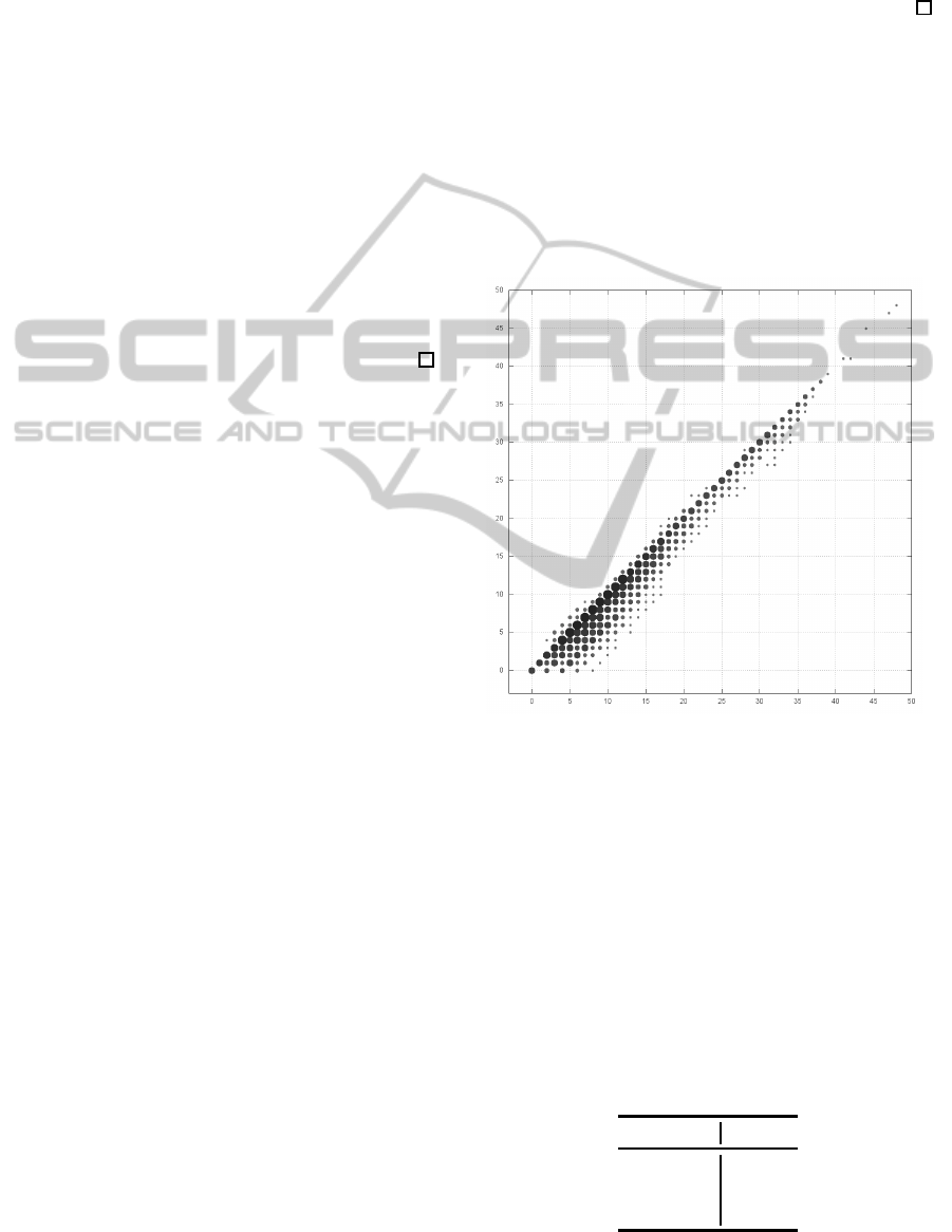
Figure 6: The correlation diagrams to the edit distance τ

TAI

of τ

ALN

for N-glycan data.

Figures 6 illustrates the correlation diagrams to

TAI

of τ

ALN

for all the 2293011 pairs of N-glycan

data. The plots in Figures 6 are the ratio (%) of the

pairs of trees whose value of τ

ALN

is given as the y-

axis to the value of τ

TAI

given in the x-axis.

Figures 6 shows that, for N-glycan data, whereas

ALN

tends to be smaller than τ

TAI

, we can observe the

pairs that τ

ALN

is greater than τ

TAI

as Proposition 5.

Table 1 represents the number of pairs comparing

ALN

with τ

TAI

in all the pairs of N-glycan data.

Table 1: The number of pairs comparing τ

ALN

with τ

TAI

case #pairs

ALN

> τ

TAI

675

ALN

= τ

TAI

1193559

ALN

< τ

TAI

298777

AlignmentofCyclicallyOrderedTrees

269

Hence, we conclude that, τ

ALN

≤ τ

TAI

for al-

most pairs of N-glycan data; Only 675 pairs (about

0.029%) satisﬁes that τ

ALN

> τ

TAI

. This result implies

that τ

ALN

(and τ

ALN

) is possible to be a good approxi-

mation of τ

TAI

for N-glycan data.

6 CONCLUSION

In this paper, we have formulated biordered, cyclic-

ordered and cyclic-biordered trees as cyclically or-

dered trees, and then designed the algorithms to com-

pute τ

ALN

, T

) and τ

SGALN

, T

) in O(nmD

) time

and to compute τ

ALN

, T

) and τ

SGALN

, T

) (π ∈

{c, cb}) in O(nmdD

) time. Finally, we have given

the experimental results of computing τ

ALN

compar-

ing with τ

TAI

by using N-glycan data.

It is a future work to implement the algo-

rithms to compute τ

ALN

, τ

ALN

and τ

SGALN

(π ∈

{b, c, cb}), and apply τ

ALN

and τ

SGALN

to real data

such as glycans (Hizukuri et al., 2005) or molecular

graphs (Horv´ath et al., 2010). Also, it is a future work

to apply cyclically ordered trees to compare RNA sec-

ondary structures (H¨ochsmann et al., 2003; Schier-

mer and Giegerich, 2013; Shapiro and Zhang, 1990;

Zhang, 1998).

As the comparison with τ

TAI

, it is a future work to

investigate how τ

ALN

(π ∈ { b, c, cb}) is a good approx-

imation of τ

TAI

and to compare τ

ALN

with tractable

variations of τ

TAI

such as the isolated-subtree dis-

tance (Zhang, 1996) and the LCA-preserving dis-

tance (Zhang et al., 1996). Also, it is a future work to

solve whether or not the problem of computing τ

ALN

is tractable if the number of permutations among sib-

lings is bounded by some polynomial with respect to

degrees.

REFERENCES

Chawathe, S. S. (1999). Comparing hierarchical data in ex-

ternal memory. In Proc. VLDB’99, pages 90–101.

Demaine, E. D., Mozes, S., Rossman, B., and Weimann, O.

(2009). An optimal decomposition algorithm for tree

edit distance. ACM Trans. Algo., 6.

Hirata, K., Yamamoto, Y., and Kuboyama, T. (2011). Im-

proved MAX SNP-hard results for ﬁnding an edit dis-

tance between unordered trees. In Proc. CPM’11

(LNCS 6661), pages 402–415.

Hizukuri, Y., Yamanishi, T., Nakamura, O., Yagi, F., Goto,

S., and Kanehisa, M. (2005). Extraction of leukemia

speciﬁc glycan motifs in humans by computational

glycomics. Carbohydrate Research, 340:2270–2278.

H¨ochsmann, M., T¨oller, T., Giegerich, R., and Kurtz, S.

(2003). Local similarity in RNA secondary structures.

In Proc. CSB’03, pages 159–168.

Horv´ath, T., Ramon, J., and Wrobel, S. (2010). Frequent

subgraph mining in outerplanar graphs. Data Min.

Knowl. Disc., 21:472–508.

Jiang, T., Wang, L., and Zhang, K. (1995). Alignment of

trees – an alternative to tree edit. Theoret. Comput.

Sci., 143:137–148.

Kan, T., Higuchi, S., and Hirata, K. (2014). Segmental

mapping and distance for rooted ordered labeled trees.

Fundamenta Informaticae, 132:1–23.

Kuboyama, T. (2007). Matching and learning in trees. Ph.D

thesis, University of Tokyo.

Lu, C. L., Su, Z.-Y., and Yang, C. Y. (2001). A new mea-

sure of edit distance between labeled trees. In Proc.

COCOON’01 (LNCS 2108), pages 338–348.

Lu, S.-Y. (1979). A tree-to-tree distance and its application

to cluster analysis. IEEE Trans. Pattern Anal. Mach.

Intell., 1:219–224.

Schiermer, S. and Giegerich, R. (2013). Forest alignment

with afﬁne gaps and anchors, applied in RNA struc-

ture comparison. Theoret. Comput. Sci., 483:51–67.

Selkow, S. M. (1977). The tree-to-tree editing problem. In-

form. Process. Lett., 6:184–186.

Shapiro, B. A. and Zhang, K. (1990). Comparing multi-

ple RNA secondary structures using tree comparision.

Comp. Appl. Biosci., 6:309–318.

Tai, K.-C. (1979). The tree-to-tree correction problem. J.

ACM, 26:422–433.

Valiente, G. (2001). An efﬁcient bottom-up distance be-

tween trees. In Proc. SPIRE’01, pages 212–219.

Wang, Y., DeWitt, D. J., and Cai, J.-Y. (2003). X-Diff: An

effective change detection algorithm for XML docu-

ments. In Proc. ICDE’03, pages 519–530.

Yamamoto, Y., Hirata, K., and Kuboyama, T. (2014).

Tractable and intractable variations of unordered tree

edit distance. Internat. J. Found. Comput. Sci.,

25:307–329.

Yoshino, T. and Hirata, K. (2013). Hierarchy of segmen-

tal and alignable mapping for rooted labeled trees. In

Proc. DDS’13, pages 62–69.

Zhang, K. (1995). Algorithms for the constrained edit-

ing distance between ordered labeled trees and related

problems. Pattern Recog., 28:463–474.

Zhang, K. (1996). A constrained edit distance between un-

ordered labeled trees. Algorithmica, 15:205–222.

Zhang, K. (1998). Computing similarity between RNA sec-

ondary structures. In Proc. IEEE Internat. Joint Symp.

Intell. Sys., pages 126–132.

Zhang, K. and Jiang, T. (1994). Some MAX SNP-hard re-

sults concerning unordered labeled trees. Inform. Pro-

cess. Lett., 49:249–254.

Zhang, K., Wang, J., and Shasha, D. (1996). On the editing

distance between undirected acyclic graphs. Internat.

J. Found. Comput. Sci., 7:43–58.

ICPRAM2015-InternationalConferenceonPatternRecognitionApplicationsandMethods

270