
Introducing the -Descriptor
A Most Versatile Relative Position Descriptor
P. Matsakis, M. Naeem and F. Rahbarnia
School of Computer Science, University of Guelph, Guelph, Canada
Keywords: Image Descriptors, Relative Position Descriptors, Spatial Relationships, F-Histograms, Affine Invariance.
Abstract: Spatial prepositions, like above, inside, near, denote spatial relationships. A relative position descriptor is a
basis from which quantitative models of spatial relationships can be derived. It is an image descriptor, like
colour, texture, and shape descriptors. Various relative position descriptors can be found in the literature. In
this paper, we introduce a new relative position descriptorthe -descriptorthat has about all the strengths of
each and every one of its competitors, and none of the weaknesses. Our approach is based on the concept of
the F-histogram and on an original categorization of pairs of consecutive boundary points on a line.
1 INTRODUCTION
The position of an object relative to another is an
important feature people rely on to understand and
communicate about space. In daily conversation,
relative positions are described through the use of
spatial prepositions, e.g., the apple in the bowl, the
bowl near the vase, the vase in front of the window.
These prepositions denote spatial relationships, which
can be categorized into topological (e.g., in), distance
(e.g., near) and directional (e.g., in front of)
relationships. From a mathematical perspective, an
object is a subset of the 2D or 3D space, and
topological relationships include set relationships.
For example, the condition AB= defines the set
(and hence topological) relationship disjoint, while
AB and int(A)int(B)= (disjoint interiors)
define the topological (but non-set) relationship
touch.
Models of spatial relationships have been
investigated in many disciplines, including cognitive
science, linguistics, geography, and artificial
intelligence. In the qualitative approach (and contrary
to the quantitative approach), the set of relationships
is discrete (not continuous); a relationship either
holds or does not hold (it cannot hold to some degree);
spatial relationship information is decoupled from the
individual features of the objects (like shape and
size). For example, in the qualitative approach, one
might consider the set {east, northeast, north,
northwest, west, southwest, south, southeast} of
directional relationships; say that the playground is
northeast of the building; argue that the exact shape
of the playground is of no importance. In the
quantitative approach, one may want to specify that
the playground is 37° east of north of the building;
allow partial truth when considering whether the
playground is northeast of the building; argue that the
shape of the playground might have an impact on the
degree to which this relationship holds. The
qualitative approach has been used extensively for
spatial reasoning, and qualitative models are by far
the most common models. However, many practical
image processing and computer vision tasks call for
quantitative models. Moreover, qualitative measures
can easily be derived from quantitative measures,
while the converse does not hold.
A relative position descriptor is an image
descriptor, and it is a basis from which quantitative
models of spatial relationships can be derived. As
such, it provides a link between low-level spatial data
features and high-level concepts. Moreover, it is a
natural complement to colour, texture, and shape
descriptors. Applications include human-robot
interaction (Skubic et al., 2004), semantic metadata
generation for image digital libraries (Wang,
Makedon, Ford et al., 2004), suspected minefield risk
estimation (Chan et al., 2005), melanocytic image
analysis and recognition (Kwasnicka and
Paradowski, 2005), geospatial information retrieval
and indexing (Shyu et al., 2007), scene matching
(Sjahputera and Keller, 2007), land cover classification
(Vaduva et al., 2010), graphical symbol retrieval
87
Matsakis P., Naeem M. and Rahbarnia F..
Introducing the Φ-Descriptor - A Most Versatile Relative Position Descriptor.
DOI: 10.5220/0005210200870098
In Proceedings of the International Conference on Pattern Recognition Applications and Methods (ICPRAM-2015), pages 87-98
ISBN: 978-989-758-076-5
Copyright
c
2015 SCITEPRESS (Science and Technology Publications, Lda.)

(Santosh et al., 2010), shape matching (Wang et al.,
2012), spatiotemporal reasoning (Salamat and
Zahzah, 2012a), and map-to-image conflation (Buck
et al., 2013).
In the light of these and other publications, here
are what seem to be the most important properties that
may be expected from a relative position descriptor.
P1 The descriptor can handle raster objects,
whatever their topology (e.g., connected or
disconnected, without or with holes), and whether
they are disjoint or not. P2 The descriptor can
handle these objects efficiently (e.g., in linear time
with respect to the number of pixels in the image). P3
The descriptor can handle vector objects. P4
The descriptor can handle distance relationships, i.e.,
meaningful distance relationship information can be
extracted in no time from the descriptor. P5 The
descriptor can handle set relationships; at the very
least, it can be used to determine whether two objects
intersect, and whether one object includes the other.
P6 The descriptor can handle topological, non-set
relationships; at the very least, it can be used to
determine whether the boundaries of two objects
intersect, and whether the interiors intersect. P7
The descriptor can handle directional relationships; at
the very least, it can be used to assess relationships
like to the right of, to the left of, above and below. P8
The descriptor can handle the relationship
surround. P9 Relative positions (as defined by the
descriptor) can be somehow compared, and similar
positions detected, regardless of which relationships
hold. P10 Given two objects A and B, the position
of B relative to A can be derived from the position of
A relative to B. P11 Given an affine transformation
t and two objects A and B, the position of t(A) relative
to t(B) can be derived from t and the position of A
relative to B. P12 Given an affine transformation t
and two objects A and
B, the transformation t can be
derived from the position of A relative to B and the
position of t(A) relative to t(B). P13 Consider four
objects A, B, A' and B' ; whether there exists an affine
transformation t such that A'=t(A) and B'=t(B) can be
derived from the position of A relative to B and the
position of A' relative to B'.
Various relative position descriptors can be found
in the literature. Most of them are histogram-based
descriptors. Each one meets a few of the above
properties. As far as we know, however, none of
them meets P1 to P13, or even P4 to P8, or P12
(Naeem and Matsakis, 2015). For example, the
histogram of forces (Matsakis and Wendling, 1999),
which is probably the relative position descriptor
backed up with the most theoretical and applied
results (Matsakis et al., 2010), does not satisfy P4-6,
P8, P12-13; the R*-histogram (Wang et al., 2004)
does not satisfy P3, P6, P8, P11-13; the spread
histogram (Kwasnicka and Paradowski, 2005) does
not satisfy P2-4, P6-7, P10-13; the radial line model
(Santosh et al., 2010) does not satisfy P4-6, P8, P11-
13; the Allen histograms (Malki et al., 2002) (Matsakis
and Nikitenko, 2005) (Salamat and Zahzah, 2012b) do
not satisfy P2, P4, P8,
P12-13; the ratio histogram
(Wang et al., 2012) does not satisfy P4-8, P12.
In this paper, we introduce a histogram-based
relative position descriptorthe -descriptor that
meets each and every one of the 13 properties.
Necessary background information is provided in
Section 2. A detailed definition of the -descriptor is
presented in Section 3. In Section 4, we briefly
explain why each property holds. Conclusions and
future work are discussed in Section 5.
2 BACKGROUND
The -descriptor is based on the concept of the F-
histogram, which is briefly reviewed in Section 2.1.
The relative position descriptor it is the closest to may
be the one defined by the Allen histograms. These
histograms are reviewed in Section 2.2 with the intent
to help the reader understand the rationale behind our
approach (Section 3).
2.1 The F-Histogram
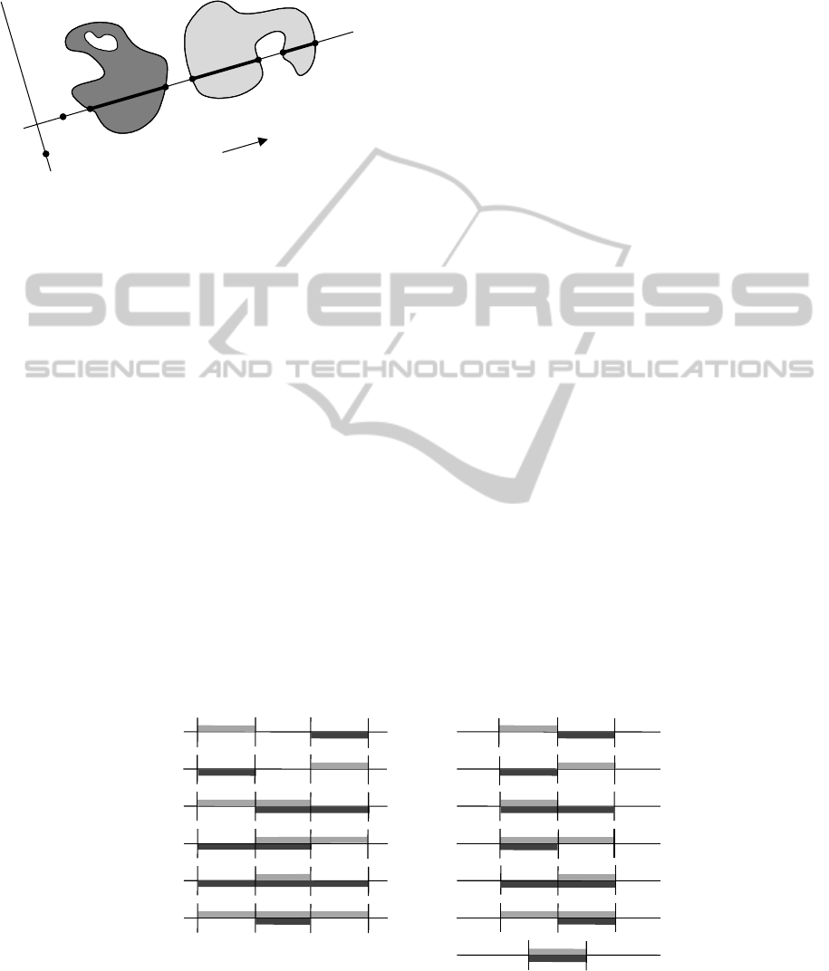
Notation and terminology are as follows. See also
Fig. 1. The symbol S denotes the Euclidean space.
The origin is an arbitrary point of S. A direction
is a unit vector. (p) is the line in direction that
passes through the point p, and
(p) is the subspace
orthogonal to that passes through p. Note that
(p)
is a line if S is of dimension 2 and is a plane if S is of
dimension 3. Now, consider a nonempty bounded
subset A of S. The intersection A(p) is a core of A.
If any core of A is a closed set with a finite number of
connected components, i.e., if it is the union of a finite
number of pairwise disjoint segments, then A is an
object. Consider a real function F that takes inputs
of the form (, S
1
, S
2
), where is a direction and S
1
and
S
2
are two subsets of S. The F-histogram associated
with the pair (A, B) of objects is the function F
AB
defined by:
(1)
F
AB
() F(, A ( p), B ( p)) dp
p
()
ICPRAM2015-InternationalConferenceonPatternRecognitionApplicationsandMethods
88
Its intended purpose is to represent, in some way, the
position of A (the argument) with respect to B (the
referent).
Figure 1: Notation: a direction , the origin , a point p, the
line (p), the orthogonal line (or plane)
(), and two
objects A and B.
The idea and assumption behind the concept of the F-
histogram (Matsakis and Wendling, 1999) (Matsakis
et al., 2010) are that acceptable representations of
relative positions can be obtained by reducing the
handling of multidimensional objects to the handling
of 1D entities. The force histogram, the R*-histogram,
the ratio histogram and the Allen histograms
mentioned in Section 1 are based on this concept.
2.2 The 13 Allen Histograms
The F-histogram naturally conveys directional
information. It is therefore tempting to use a fuzzy
approach and choose the function F such that the real
number F(, A(p), B(p)) measures the extent to
which a given topological relationship holds
between A(p) and B(p). If there are n possible
topological relationships between two such cores, n
histograms (one per relationship) should convey com-
prehensive quantitative information on the directional
and topological relationships between the two objects
A and B. Unfortunately, there are infinitely many
binary relations definable in the algebra generated by
unions of segments on a directed line (Ladkin, 1986).
In the simple case of a segment and the union of two
disjoint segments, there are already over 40
topological relationships (Egenhofer, 2007). It seems
wise to avoid a combinatorial explosion and rely on
the very well known 13 Allen relations between two
segments (Allen, 1983). See Fig. 2. For every
segment (i.e., connected component) I of A(p)
and for every segment J of B(p), the value F(, I,
J) then measures the extent to which a given
(fuzzified) Allen relation holds between I and J; as for
F(, A(p), B(p)), it is some aggregate of all the
F(, I, J) values.
There are several issues with this approach, which
has been explored in various publications (Malki et
al., 2002) (Matsakis and Nikitenko, 2005) (Salamat
and Zahzah, 2012b). For example, it is hard to extract
meaningful 2D topological relationship information
from the 13 histograms of 1D fuzzy Allen relations,
especially when the objects are not convex. This is
apparent in (Matsakis et al., 2010) (Salamat and
Zahzah, 2012c). Moreover, it is often impossible to
extract crisp topological relationship information. To
illustrate this, let F
P
and F
M
be the functions F
attached to the Allen relations P (precedes) and M
(meets). Assume
F
P
AB
() 0
and
F
M
AB
() 0
. It may
be because the statements “A(p
1
) precedes
B(p
1
)” and “A(p
2
) meets B(p
2
)” are both
totally true (and AB). However, since P and M
are conceptual neighbours and have been fuzzified, it
may also be because the statements “A(p) precedes
B(p)” and “A(p) meets B(p)” are both
partially true (and AB=). As a result, one cannot
answer with ‘yes’ or ‘no’ the question: “Are these
objects disjoint?”
Figure 2: The 13 relations between two aligned segments (Allen, 1983). In each case, the argument is the light gray segment
and the referent is the dark gray segment. P=Precedes, M=Meets, O=Overlaps, S=Starts, D=During, F=Finishes, E=Equals,
Pi=P-inverse=Preceded by, Mi=Met by, Oi=Overlapped by, Si=Started by, Di=Contains, Fi=Finished by.
B
A
ω
θ
p
θ (ω)
T
θ(p)
P
Pi
O
Oi
D
Di
M
Mi
S
Si
F
Fi
E
IntroducingthePhi-Descriptor-AMostVersatileRelativePositionDescriptor
89
3 DEFINITION
The -descriptor is built upon 13 F-histograms. Each
histogram value corresponds to the area (in dimension
2) or volume (in dimension 3) of a region delimited
by parallel lines and the boundaries of the objects in
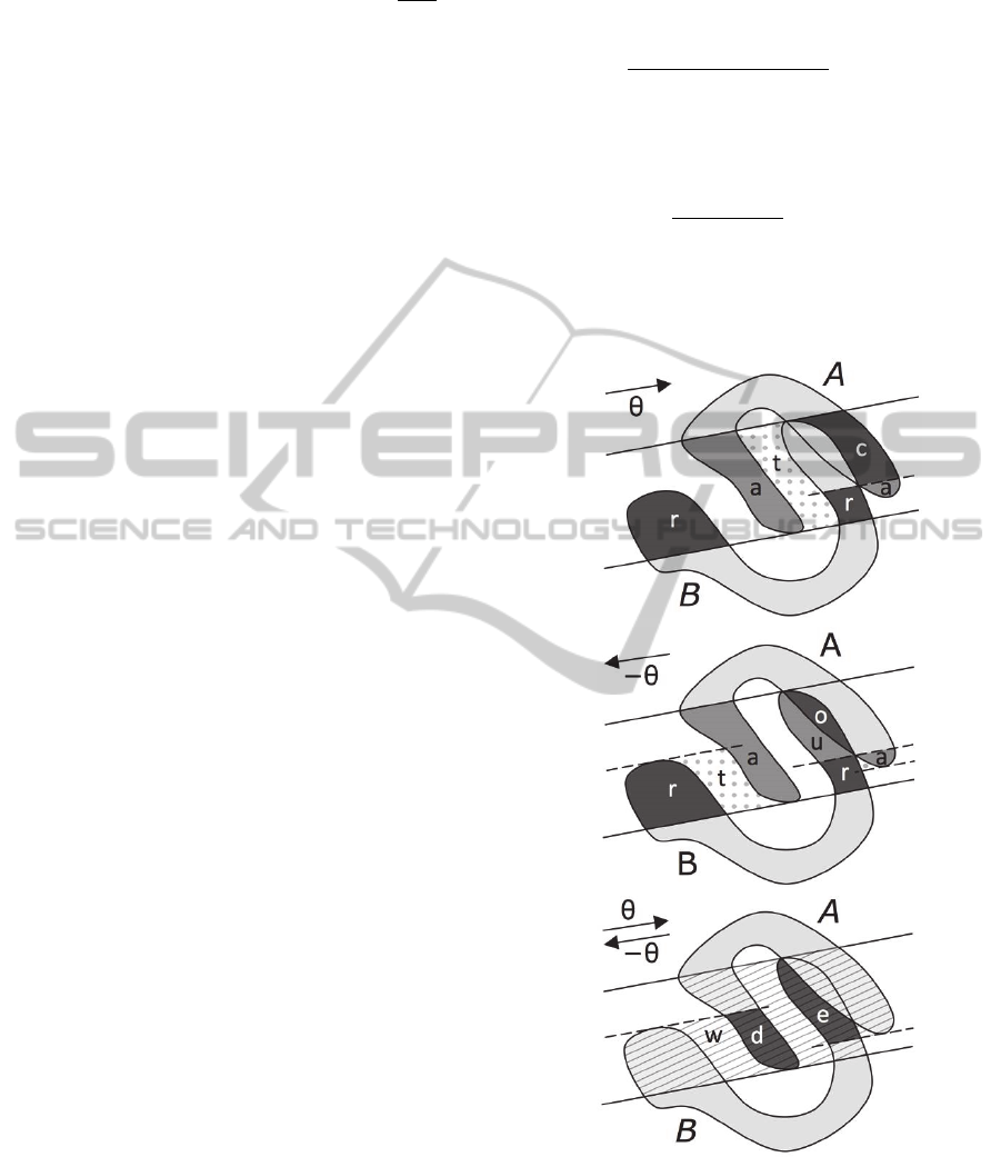
hand (Fig. 3). The outline of this section is as follows:
a directed straight line intersects the boundaries of
two objects in several points; these points fall into 12
categories, and the pairs of consecutive points fall into
36 categories (Section 3.1) divided into 10 groups
(Section 3.2); a function is attached to each group and
maps each pair to a real number; the 10 functions and
3 others are used to define the 13 F-histograms
(Section 3.3) that are the basis of the -descriptor
(Section 3.4).
3.1 Boundary Points and Categories
Let A and B be two objects and let be a direction.
Consider a line L in direction . Its intersection with
A has a finite number of connected components, and
each component is a line segment. Let p and q be the
endpoints of one of these segments. If pq and
pq/|pq|=, where pq denotes the vector from p to q
and |pq| denotes its length, then p is an A-entry (on L,
in direction ) and q is an A-exit. Now, consider the
set {p
1
, p
2
, …, p
n
} of all A-entries, A-exits, B-entries
and B-exits on L and in direction . Assume that for
any i we have p
i
p
i+1
/|p
i
p
i+1
|=. The point p
i+1
is then
the successor of p
i
. See Fig. 4. Consider two elements
p and q of {p
1
, p
2
, …, p
n
} such that q is the successor
of p. The point p falls into one of 12 categories, which
can be named and represented as in Fig. 5. The same
applies to q. As a result, the pair (p,q) falls into one of
36 categories. These categories, numbered from 1 to
36, are shown in Fig. 6. They may remind the reader
of the Allen’s relations. The two concepts are, in a
sense, the reverse of each other: an Allen relation
involves 2 segments, and up to 4 distinct points are
the endpoints of these segments (Fig. 2); on the other
hand, a point pair category involves 2 distinct points,
and up to 4 segments have these points as endpoints.
3.2 Grouping the Point Pair Categories
In Fig. 6, the 36 point pair categories are divided into
9 groups (A-A, B-B, A-B, etc.). The division was
convenient when trying to list all the categories. In
this section, however, other groups are considered.
Seven are labeled with a verb (third person singular
form in the simple present tense): trails, overlaps,
covers, uncovers, follows, leads, or starts. See Fig. 7.
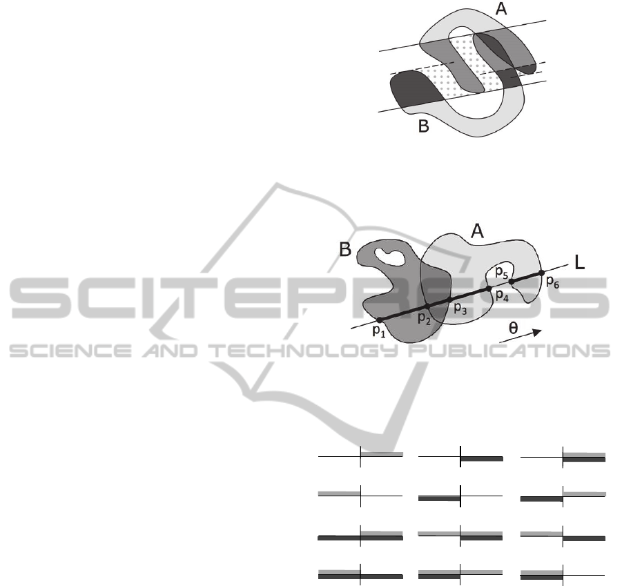
Figure 3: A glimpse into the area F-histograms. Each
histogram value corresponds to the area of a region. Ten
such regions are represented here (medium gray, dark gray,
and dotted regions).
Figure 4: Entry and exit points. On L, in direction , the
point p
1
is a B-entry not in A, the point p
2
is an A-entry in B,
etc. (see Fig. 5); the pair (p
1
,p
2
) falls into the category 13,
the pair (p
2
, p
3
) into the category 11, etc. (see Fig. 6).
Figure 5: The 12 point categories. In each case, the
argument is the light gray segment and the referent is the
dark gray segment.
Each verb indicates a particular relationship between
a segment of the argument A and a segment of the
referent B. For example, in categories 10, 18, 32 and
36 a segment of A (left) is far behind (i.e., trails) a
segment of B (right), while in categories 26, 30 and
34 a segment of A (left) is right behind (i.e., follows)
a segment of B (center). Note that the terms overlaps,
follows and starts are commonly used to denote the
Allen relations O, F and S (Fig. 2). The reader should
assume their meaning here is unrelated. Three
groups of categories are labeled with a noun: void,
argument, or referent. See Fig. 8. In these categories,
there is no useful relationship between a segment of
A‐entry
not
in
B
A‐exit
not
in
B
A‐entry
in
B
A‐exit
in
B
B‐entry
not
in
A
B‐exit
not
in
A
B‐entry
in
A
B‐exit
in
A
A‐entry
B‐entry
A‐entry
B‐exit
A‐exit
B‐entry
A‐exit
B‐exit
ICPRAM2015-InternationalConferenceonPatternRecognitionApplicationsandMethods
90
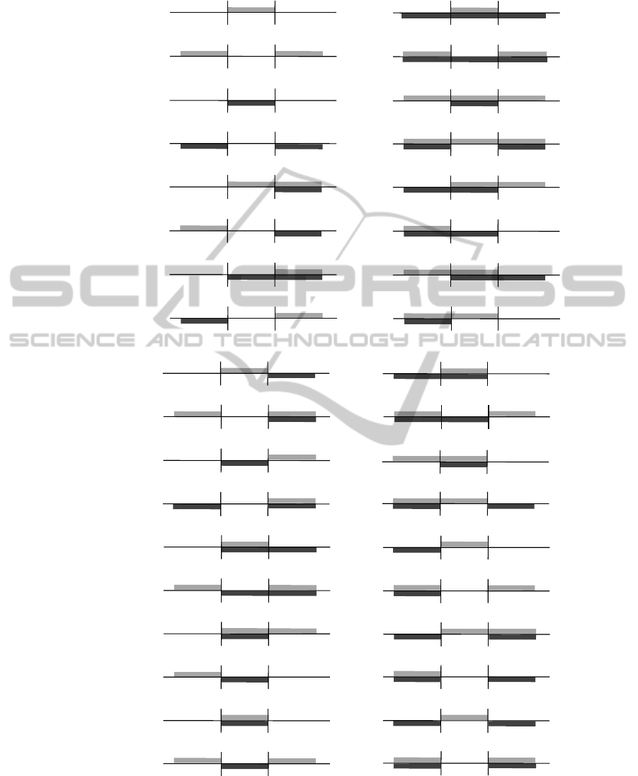
Figure 6: The 36 point pair categories. They are here divided into 9 groups of 4 categories. For example, AB-B means that
the first point p is an A-entry or A-exit and a B-entry or B-exit, while its successor q is a B-entry or B-exit only. In each case,
the argument is the light gray segment and the referent is the dark gray segment.
A‐A
overlaps
argument
void
referent
1
2
3
4
A‐B
B‐A
trails
uncovers
covers
overlaps
(covers)
(overlaps)
(uncovers)
(trails)
9
10
13
14
11
12
15
16
B‐B
overlaps
argument
void
referent
5
6
7
8
AB‐A
AB‐B
A‐AB
B‐AB
AB‐AB
trails
starts
follows
leads
starts
starts
trails
trails
follows
leads
follows
leads
(leads)
(follows)
(trails)
(starts)
(follows)
(starts)
(leads)
(trails)
17
18
21
22
25
26
29
30
33
34
19
20
23
24
27
28
31
32
35
36
IntroducingthePhi-Descriptor-AMostVersatileRelativePositionDescriptor
91
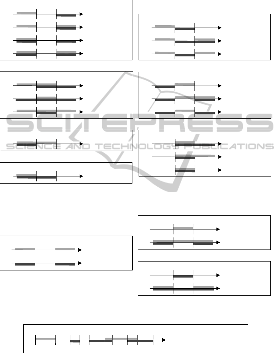
Figure 7: Nonzero values for the functions f
t
, f
o
, f
c
, f
u
, f
f
, f
and f
s
.
Figure 8: Nonzero values for the functions f
v
, f
a
and f
r
.
Figure 9: Nonzero values for the functions f
e
, f
d
and f
w
. Examples.
p
q
f
t
(θ,p,q)=|pq|
f
t
(θ,p,q)=|pq|
trails
f
t
(θ,p,q)=|pq|
f
t
(θ,p,q)=|pq|/2
p
q
f
c
(θ,p,q)=|pq|
covers
p
q
f
u
(θ,p,q)=|pq|
uncovers
p
q
f
f
(θ,p,q)=|pq|
f
f
(θ,p,q)=|pq|
f
f
(θ,p,q)=|pq|/2
follows
p
q
f
(θ,p,q)=|pq|
f
(θ,p,q)=|pq|
f
(θ,p,q)=|pq|/2
leads
p
q
f
s
(θ,p,q)=|pq|
f
s
(θ,p,q)=|pq|
f
s
(θ,p,q)=|pq|/2
starts
p
q
f
o
(θ,p,q)=|pq|
f
o
(θ,p,q)=|pq|/2
f
o
(θ,p,q)=|pq|/2
overlaps
10
18
32
36
15
3
7
16
12
30
26
34
27
31
35
25
29
33
θ
θ
θ
θ
θ
θ
θ
p
q
f
v
(θ,p,q)=|pq|/2
f
v
(θ,p,q)=|pq|/2
void
p
q
f
a
(θ,p,q)=|pq|/2
f
a
(θ,p,q)=|pq|/2
argument
p
q
f
r
(θ,p,q)=|pq|/2
f
r
(θ,p,q)=|pq|/2
referent
2
6
1
8
5
4
θ
θ
θ
p
1
p
2
p
3
p
4
p
5
p
6
p
7
p
8
p
9
p
10
f
e
(θ,p
2
,p
6
)=|p
3
p
4
|+|p
5
p
6
|
f
d
(θ,p
7
,p
8
)=|p
7
p
8
|
f
w
(θ,p
1
,p
10
)=|p
1
p
10
|
encloses,
divides,
width
θ
ICPRAM2015-InternationalConferenceonPatternRecognitionApplicationsandMethods
92

A and a segment of B. Each noun refers to the object
(if any) that occupies the space between p and q.
Finally, note that the 10 groups shown in Figs. 7 and
8 include 24 categories only (instead of 36). Twelve
are ignored to avoid redundancy and keep
information directional; in Fig. 6, these categories are
labeled with names in brackets. For example,
category 9 is ignored because it is the directional
inverse of category 16: if p is a B-exit and q an A-exit
on line L and in direction (category 16), then q is an
A-entry and p a B-entry on line L and in direction
(category 9).
3.3 Area and Volume F-Histograms
Consider two objects A and B. First, we define 10 real
functions f
t
, f
o
, f
c
, f
u
, f
f
, f
, f
s
, f
v
, f
a
and f
r
(the subscript
t stands for trails, o for overlaps, c for covers, etc.).
These functions take inputs of the form (,p,q), where
is a direction and p and q are two points. Let L be
the line in direction that passes through p. Assume
{p
1
, p
2
, …, p
n
} is the set of all A-entries, A-exits, B-
entries and B-exits on L and in direction , as in
Section 3.1. Each function f maps (,p,q) to 0 unless
(p,q) is a pair (p
i
,p
i+1
) that falls into a category f is
attached to. In that case, we have f(,p,q)=|pq| (and
f(,q,p)=0) if the category is not its own directional
inverse; we have f(,p,q)=|pq|/2 (and
f(,q,p)=|pq|/2) otherwise. See Figs. 7 and 8. In a
nutshell, the greater the distance between p and q, the
more a segment of A trails, or overlaps, covers, etc.,
a segment of B.
We now define 3 more functions: f
e
, f
d
and f
w
. The
reason for this will be clarified later. The value
f
e
(,p,q) is 0 unless (p,q) is a pair (p
i
,p
j
) with j>i, the
point p
i
is an A-exit, pj is an A-entry, and for any k in
the integer interval i+1..j1 the point p
k
is neither an
A-exit nor an A-entry; in that case, f
e
(,p,q) is the total
length of B[p
i
,pj]. The value f
d
(,p,q) is 0 unless
(p,q) is a pair (p
i
,p
j
) with j>i, the point p
i
is a B-exit,
p
j is a B-entry, and for any k in i+1..j1 the point p
k
is
neither a B-exit nor a B-entry; in that case, f
d
(,p,q) is
the total length of A[p
i
,pj]. Finally, the value
f
w
(,p,q) is 0 unless (p,q) is the pair (p
1
,p
n
); in that
case, f
w
(,p,q)=|p
1
p
n
|. See Fig. 9.
The next step is to define 13 other functions F
t
,
F
o
, F
c
, F
u
, F
f
, F
l
, F
s
, F
v
, F
a
, F
r
, F
e
, F
d
and F
w
. Each
one maps (, AL, BL) to 0 if the set of all A-entries,
A-exits, B-entries and B-exits on L and in direction
is empty. Otherwise:
F
t
(, A L, B L) f
t
(,p
i
,p
i+1
)
i
1
n1
(2)
F
o
(, A L, B L) f
o
(,p
i
,p
i+1
)
i
1
n1
(3)
…
(4-10)
F
r
(, A L, B L) f
r
(,p
i
,p
i+1
)
i
1
n1
(11)
F
e
(,A L, B L) f
e
(,p
i
,p
j
)
ji1
n
i1
n
1
(12)
F
d
(, A L, B L) f
d
(,p
i
,p
j
)
ji1
n
i1
n
1
(13)
F
w
(
, A
L, B
L)
f
w
(
,p
1
,p
n
)
(14)
These functions F and (1) allow us to define 13 F-
histograms:
F
t
AB
,
F
o
AB
,
F
c
AB
,
F
u
AB
,
F
f
AB
, F
A B
,
F
s
AB
,
F
v
AB
,
F
a
AB
,
F
r
AB
,
F
e
AB
,
F
d
AB
,
F
w
AB
.
Each histogram value corresponds to an area (in
dimension 2) or volume (in dimension 3). See Fig. 10.
Note that
F
w
AB
()
is the area or volume of the region
of interaction in direction .
3.4 Length Histograms and the
-Descriptor
Let be the real function of a real variable defined by
(0)=0 and (x)=1 if x0. The length histogram
F
w
AB
is the real function defined by Equation (15).
F
w
AB
()
=
F
w
AB
()
(F
w
(, A( p), B(p))) dp
p
()
(15)
F
w
AB
()
is the average width of the region of
interaction in direction . We may also say that it is
the average nonzero f
w
value in direction . Note that
F
w
AB
is undefined at if
F
w
AB
()
= 0. Likewise, we
can define the length histograms
F
t
AB
,
F
o
AB
, etc. For
example,
F
t
AB
()
is the average nonzero f
t
value in
direction .
We can now introduce the -descriptor associated
with the pair (A, B) of objects. It is a tuple
AB
of area
(dimension 2) or volume (dimension 3) F-
histograms and of length histograms. Its intended
purpose is to represent the position of A relative to B.
One possible definition is given by Equation (16),
although more length histograms may be considered.
measure(A) denotes the area (dimension 2) or the
volume (dimension 3) of A. Note that
F
w
AB
can
actually be derived from
F
t
AB
,
F
o
AB
, …,
F
r
AB
.
IntroducingthePhi-Descriptor-AMostVersatileRelativePositionDescriptor
93
AB
= (
F
t
AB
,
F
o
AB
,
F
c
AB
,
F
u
AB
,
F
f
AB
, F
A B
,
F
s
AB
,
F
v
AB
,
F
a
AB
,
F
r
AB
,
F
e
AB
,
F
d
AB
,
F
w
AB
,
F
w
AB
,
measure(A),
measure(B) ) (16)
4 PROPERTIES
The -descriptor satisfies each and every one of the
properties P1 to P13 (Section 1). In this section, we
briefly explain why. Complete proofs are given in
separate papers, including (Matsakis and Naeem,
submitted). Although the definition of the -
descriptor holds in any Euclidean space, it is assumed
here that S is of dimension 2.
4.1 P1 to P3, P9 and P10 (Basics)
P1 and P2 In the case of raster objects, the -
descriptor, which has obviously been designed with
arbitrary objects in mind, can be computed in a very
efficient way. For every direction , the image is
partitioned into parallel raster lines. The pixels in a
line are examined one by one and all the
F
AB
()
and
F
AB
()
values are updated on the fly; basically, it is
just a matter of counting the number of pixels
between every two consecutive entry or exit points
(i.e., boundary pixels). In the end, the -descriptor is
computed in (KN) time, where N is the number of
pixels in the image and K is the number of directions
considered. Note that the higher K, the more
complete the collected histogram data, but the longer
the processing time. Practically, there does not seem
to be any interest in considering more than a few
hundred directions when computing F-histograms,
and K is chosen between 4 and 360 (Matsakis et al.
2010).
P3 In the case of vector objects, updating the
F
AB
()
and
F
AB
()
values comes down to calculating
the areas of polygons delimited by the boundaries of
the objects and lines in direction . The -descriptor
is computed in (K
3
) time, where is the total
number of object vertices. However, this worst-case
performance falls to (K
2
) when the objects
intersect in points or less, which is typical in
practice.
P9 A simple way to compare two relative
positions
AB
and
A’B’
is to compare their
corresponding elements, i.e.,
F
t
AB
with
F
t
A' B'
,
F
o
AB
with
F
o
A' B'
, etc. For example, the similarity between two
histograms h
1
and h
2
can be calculated using a
measure introduced by Pappis and Karacapilidis
(1993):
min{h
1
(), h
2
()}
max{h
1
(), h
2
()}
(17)
Likewise, the similarity between two object areas a
1
and a
2
can be evaluated as:
min{a
1
,a
2
}
max{a
1
,a
2
}
(18)
The similarity, sim, between
AB
and
A’B’
can then
be defined as the minimum similarity between
corresponding histograms and object areas.
(a)
(b)
(c)
Figure 10: Area F-histogram values. For example,
F
r
AB
()
is
half the total area of the two regions in (a) labeled r, and
F
r
AB
()
=
F
r
AB
()
; the value
F
u
AB
()
is 0, but
F
u
AB
()
is the
area of the region in (b) labeled u; the value
F
w
AB
()
is the
area of the region in (c) filled with diagonal lines, and
F
w
AB
() F
w
AB
()
.
ICPRAM2015-InternationalConferenceonPatternRecognitionApplicationsandMethods
94
P10 Each
F
BA
or
F
BA
histogram can be
derived from an
F
AB
or
F
AB
histogram. For
example, for any direction , we have
F
t
BA
() F
t
AB
()
and
F
c
BA
() F
u
AB
()
. As a
result, the position of B relative to A can be derived
from the position of A relative to B.
4.2 P4 to P8 (Spatial Relationships)
A great amount of spatial (including topological,
directional and distance) relationship information
can be extracted from the -descriptor. For example,
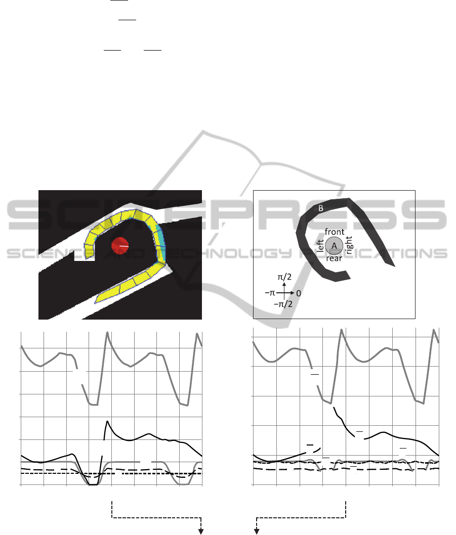
consider Fig.
11. Figure 11a is a world view of a robot
in an environment with corridors and doorways. The
robot is a mobile Nomad 200 with 16 sonar sensors
evenly distributed along its circumference. The
sensor readings were used to build an approximate
polygonal representation of the surrounding
obstacles. The experiment was done using the
Nomadic simulator. Figure 11b shows an egocentric
robot view of the scene. The position of A (the robot)
relative to B (the perceived environment) is
described using the -descriptor. See Figs. 11cd.
Since
F
o
AB
=
F
s
AB
=0 (everywhere zero histograms),
the interiors of A and B do not intersect (this is good
news for the robot). Moreover, since
F
f
AB
=F
A B
=0,
the objects A and B do not even touch; they are
disjoint (the robot is not leaning against the wall). The
average distance, in direction , between A and B is
(a) (b)
(c) (d)
RobottoHuman:“Iampartiallysurroundedbyobstacles.
Theclosestobstacleisonmyrear‐left.
Thereisanopeningonmyrear‐right.”
Figure 11: (a) A robot with sonar sensors, its environment, and its perception of the environment (Skubic et al., 2003). (b) An
egocentric robot view of the scene. (c) The corresponding area histograms (w for
F
w
AB
, t for
F
t
AB
, etc.), and (d) the
corresponding length histograms. On the vertical axes, area(A) denotes the area of A while diam(A) denotes its diameter.
3
area(A)
0
−π/2
0
π/2
π
d
w
r
a
6
area(A)
−π
t
4 diam(A)
2 diam(A)
0
−π/2
0
π/2
π
−π
t
w
r
t
d
a
IntroducingthePhi-Descriptor-AMostVersatileRelativePositionDescriptor
95
F
t
AB
()
; it is minimum when =3/4 (on the robot’s
rear-left). The object A would be totally surrounded
by B if we had
F
d
AB
()
= area(A) for all , but this is
not the case. However, A is partially surrounded by
B, since
F
d
AB
()
= area(A) for all in the interval
[0,/2] and
F
d
AB
()
0 for all in [/8, 5/8]. There
is a /8-wide opening in direction /4 (on the robot’s
rear-right), since
F
d
AB
and
F
t
AB
are 0 on [/4,/8].
Note that Fig. 11b may be seen as an illustration
of one of the RCC23 spatial relationships (Cohn et al.
1997): the objects A and B do not intersect (AB =),
the convex hull of A does not intersect B
(conv(A)B=), and the convex hull of B includes A
(conv(B)A=A). The -descriptor is able to identify
every single one of the RCC23 relationships (and
many, many more). In other words, it is able to
provide crisp information and indicate whether yes or
no a given relationship holds. With all the numerical
histogram values available, it is also able, of course,
to provide fuzzy information and indicate to what
extent one may say that the relationship holds.
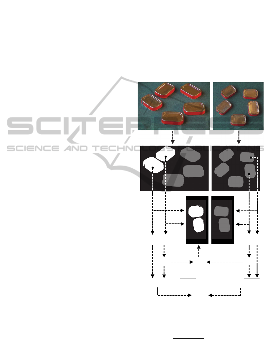
4.3 P11 to P13 (Affine Transformations)
Consider Fig. 12. Figures 12ab show two RGB
pictures taken with a commercial digital camera,
while Figs. 12cd show the pictures after
segmentation. Segmentation was achieved by
choosing the color channel with the best contrast (red
channel), running an optimum thresholding algorithm
(like Otsu’s) on the corresponding gray-level
histogram, and performing 7x7 median filtering on
the thresholded image. Are the RGB pictures two
pictures of the same scene? If so, which can (Figs.
12ac) is which (Figs. 12bd)? Color, texture, and shape
descriptors would clearly not be very helpful in
answering these questions. Later in this section, we
focus on the two cans A
1
and A
2
, and we use this
matching problem to illustrate the affine
transformation properties of the -descriptor.
Affine invariant descriptors play an important role
in computer vision. Examples of affine invariant
colour, texture, and shape descriptors abound in the
literature. The -descriptor can be normalized to
obtain affine invariance and has many interesting
related properties. Let aff be an invertible affine
transformation. Areas under an affine transformation
are scaled by the absolute value of the determinant of
the matrix that represents the linear part of the affine
transformation. As a result,
aff(A)aff(B)
can be easily
derived from aff and
AB
. In other words, the
behaviour of the -descriptor under affine
transformations is known.
We have developed a normalization procedure
AB
AB
with the two following properties.
Except for particular object pairs (i.e., object pairs
that are not well-behaved), there exists a unique
invertible linear transformation lin such that:
AB
=
lin(A)lin(B)
(19)
Moreover, for any well-behaved object pair and for
any invertible affine transformation aff we have:
Figure 12: (a)(b) Two RGB pictures. (c)(d) The pictures
after segmentation. According to the -descriptor, the best
match for (A
1
,A
2
) is (B
3
,B
4
), and the linear transformation that
best changes (A
1
,A
2
) into (B
3
,B
4
) is lin.
aff ( A) aff ( B)
=
AB
(20)
In other words, the normalized -descriptor is affine
invariant. The idea behind -descriptor
Φ
A
A
1 2
lin(A
1
)
lin(A
2
)
A
1
A
2
A
3
A
4
A
5
B
1
B
2
B
3
B
4
B
5
Φ
B
B
3
4
B
3
B
4
Φ
lin
(A
)
lin
(A
)
=
A
1
A
2
lin
A
Φ
A
A
1 2
Φ
lin
(B
)
lin
(B
)
=
B
3
B
4
Φ
B
B
3
4
lin
B
lin
sim
(a) (b)
(c) (d)
ICPRAM2015-InternationalConferenceonPatternRecognitionApplicationsandMethods
96

normalization is to derive from
AB
a vector basis
intrinsic to the pair (A,B). The uniqueness of lin
comes from the uniqueness of the transformation used
to change a vector basis into another. Note that the
normalization procedure involves the length
histogram
F
w
AB
and uses the fact that the behaviour
of the -descriptor under affine transformations is
known. Consider Fig. 12 again:
A
1
A
2
is derived from
A
1
and A
2
; then, lin
A
is derived from
A
1
A
2
; finally,
A
1
A
2
is derived from lin
A
and
A
1
A
2
.
Now, let (A,B) and (A',B') be two well-behaved
object pairs. If there exists an invertible affine
transformation aff such that
A' = aff(A) and B' = aff(B) (21)
then aff can be easily retrieved (up to a translation)
from
AB
and
A’B’
, using the normalization
procedure. Moreover, if there exists an invertible
transformation t (not necessarily affine) such that
A' = t(A) and B' = t(B) (22)
then the linear transformation that best approximates
t (up to a translation) can be found, and the quality of
the approximation can be assessed. Consider Fig. 12
once again: lin
A
is derived from
A
1
A
2
and lin
B
is
derived from
B
3
B
4
; then lin is derived from lin
A
and
lin
B
. In this case, however, (A
1
,A
2
) and (B
3
,B
4
) are not
affine-related (although they are matching pairs): in
photography, the image formation process involves
projective transformations instead of affine
transformations; besides, A
1
, A
2
, B
3
and B
4
are 2D
representations of 3D cans. The linear transformation
lin is, therefore, only an approximation of the non-
affine transformation that changes (A
1
,A
2
) into
(B
3
,B
4
). Compare (lin(A
1
),lin(A
2
)) with (B
3
,B
4
). To
assess the quality of the approximation, one must
compare the two normalized descriptors
A
1
A
2
and
B
3
B
4
, i.e., calculate their similarity sim (see Section
4.1, Property P9). Note that the similarity between
A
1
A
2
and
B
i
B
j
, where i and j belong to {1,2,3,4,5},
was found to be maximum for i=3 and j=4.
5 CONCLUSIONS
What are the most important properties that may be
expected from a relative position descriptor? In the
light of articles on these descriptors and their
applications, we have identified 13 properties. Taken
individually, the current descriptors meet only a few
of them. In this paper, we have introduced a relative
position descriptorthe -descriptorthat meets
each and every one of the 13 properties.
While most descriptors reduce the study of the
relative position between two objects to the study of
the relative positions between elementary
components of the objects (e.g., pixels, points,
segments), the -descriptor uses an original approach
based on the categorization of pairs of consecutive
boundary points on a line. Moreover, the -descriptor
consists of raw data that are easy to acquire and
interpret. There is no time-consuming pre-
processing, like force calculation, or membership
degree calculation. More spatial relationship
information is preserved and can be extracted.
We are now developing a library of crisp and
fuzzy models of spatial relationships based on the -
descriptor. The next step will be to focus on 3D
objects; the definition of the -descriptor holds in any
Euclidean space, but only 2D objects have been
considered so far. As for fuzzy objects, they can be
handled using, e.g., the double sum scheme by Dubois
and Jaulent (1987), or the simple sum scheme by
Krishnapuram et al. (1993). However, such generic
schemes are computationally expensive. Since the
elementary values of the -descriptor are areas, there
should be a much simpler and more efficient way to
process fuzzy objects, based on the concept of the area
of a fuzzy set. The idea will have to be validated.
REFERENCES
J. F. Allen, 1983. “Maintaining Knowledge About
Temporal Intervals,” Communications of the ACM,
26(11): 832-43.
A. Buck, J. M. Keller, M. Skubic, 2013. “A Memetic
Algorithm for Matching Spatial Configurations with the
Histograms of Forces,” IEEE Trans. on Evolutionary
Computation, 17(4):588-604.
J. C.-W. Chan, H. Sahli, Y. Wang, 2005. “Semantic Risk
Estimation of Suspected Minefields Based on Spatial
Relationships Analysis of Minefield Indicators from
Multi-Level Remote Sensing Imagery,” Detection and
Remediation Technologies for Mines and Minelike
Targets X, Proceedings of SPIE, 5794(1):1071-9.
A. G. Cohn, B. Bennett, J. Gooday, N. M. Gotts, 1997.
“Qualitative Spatial Representation and Reasoning with
the Region Connection Calculus,” GeoInformatica,
1(3):275-316.
D. Dubois, M.-C. Jaulent, 1987. “A General Approach to
Parameter Evaluation in Fuzzy Digital Pictures,”
Pattern Recognition Letters, 6:251-59.
M. J. Egenhofer, 2007. “Temporal Relations of Intervals
with a Gap,” 14th Int. Symposium on Temporal
Representation and Reasoning, Proceedings, 169-74.
IntroducingthePhi-Descriptor-AMostVersatileRelativePositionDescriptor
97

R. Krishnapuram, J. M. Keller, Y. Ma, 1993. “Quantitative
Analysis of Properties and Spatial Relations of Fuzzy
Image Regions,” IEEE Trans. on Fuzzy Systems, 1(3):
222-33.
H. Kwasnicka, M. Paradowski, 2005. “Spread Histogram
A Method for Calculating Spatial Relations Between
Objects,” 4th Int. Conf. on Computer Recognition
Systems (CORES), Proceedings, 30:249-56.
P. Ladkin, 1986. The Logic of Time Representation, PhD
Thesis, University of California at Berkeley.
J. Malki, E.-H. Zahzah, L. Mascarilla, 2002. “Indexation et
recherche d'image fondées sur les relations spatiales
entre objets,” Traitement du Signal, 18(4):235-51.
P. Matsakis, M. Naeem, submitted. “Basic and Affinity-
Related Properties of a Groundbreaking Relative
Position Descriptor,” IEEE Trans. on Pattern Analysis
and Machine Intelligence.
P. Matsakis, D. Nikitenko, 2005. “Combined Extraction of
Directional and Topological Relationship Information
from 2D Concave Objects,” in M. Cobb, F. Petry, V.
Robinson (Eds.), Fuzzy Modeling with Spatial
Information for Geographic Problems, Springer-Verlag,
15-40.
P. Matsakis, L. Wawrzyniak, J. Ni, 2010. “Relative
Positions in Words: A System that Builds Descriptions
Around Allen Relations,” Int. J. of Geographical
Information Science, 24(1):1-23.
P. Matsakis, L. Wendling, 1999. “A New Way to Represent
the Relative Position of Areal Objects,” IEEE Trans. on
Pattern Analysis and Machine Intelligence, 21(7):634-
43.
P. Matsakis, L. Wendling, J. Ni, 2010. “A General
Approach to the Fuzzy Modeling of Spatial
Relationships,” in R. Jeansoulin, O. Papini, H. Prade,
S. Schockaert (Eds.), Methods for Handling Imperfect
Spatial Information, Springer-Verlag, 49-74.
M. Naeem, P. Matsakis, 2015, “Relative Position
Descriptors: A Review,” 4th Int. Conf. on Pattern
Recognition Applications and Methods, Proceedings, in
press.
C. Pappis, N. Karacapilidis, 1993. “A Comparative
Assessment of Measures of Similarity of Fuzzy
Values,” Fuzzy Sets and Systems, 56:171-4.
N. Salamat, E.-H. Zahzah, 2012a. “Spatio-Temporal
Reasoning by Combined Topological and Directional
Relations Information,” Int. J. of Artificial Intelligence
and Soft Computing, 3(2):185-201.
N. Salamat, E.-H. Zahzah, 2012b. “On the Improvement of
Combined Fuzzy Topological and Directional
Relations Information,” Pattern Recognition,
45(4):1559-1568.
N. Salamat, E.-H. Zahzah, 2012c. “Two-Dimensional
Fuzzy Spatial Relations: A New Way of Computing and
Representation,” Advances in Fuzzy Systems, 2012: 1-15.
K.C. Santosh, L. Wendling, B. Lamiroy, 2010. “Unified
Pairwise Spatial Relations: An Application to
Graphical Symbol Retrieval,” in J.-M. Ogier, W. Liu,
J. Llados (Eds.), Graphics Recognition.
Achievements, Challenges, and Evolution, Springer-
Verlag, 163-74.
C.-R. Shyu, M. Klaric, G. J. Scott, A. S. Barb, C. H. Davis,
K. Palaniappan, 2007. “GeoIRIS: Geospatial
Information Retrieval and Indexing System Content
Mining, Semantics Modeling, and Complex Queries,”
IEEE Trans. on Geoscience and Remote Sensing,
45(4):839-52.
O. Sjahputera, J. M. Keller, 2007. “Scene Matching Using
F-Histogram-Based Features with Possibilistic C-Means
Optimization,” Fuzzy Sets and Systems, 158(3):253-69.
M. Skubic, P. Matsakis, G. Chronis, J. M. Keller, 2003.
“Generating Multi-Level Linguistic Spatial Descriptions
from Range Sensor Readings Using the Histogram of
Forces,” Autonomous Robots, 14(1):51-69.
M. Skubic, D. Perzanowski, S. Blisard, A. Schultz, W.
Adams, M. Bugajska, D. Brock, 2004. “Spatial
Language for Human-Robot Dialogs,” IEEE Trans. on
Systems, Man, and Cybernetics (Part C), 34(2):154-67.
C. Vaduva, D. Faur, I. Gavat, 2010. “Data Mining and
Spatial Reasoning for Satellite Image
Characterization,” 8th Int. Conf. on Communications
(COMM), Proceedings, 173-176.
Y. Wang, F. Makedon, A. Chakrabarti, 2004. “R*-
Histograms: Efficient Representation of Spatial
Relations between Objects of Arbitrary Topology,”
12th Annual ACM Int. Conf. on Multimedia (MM),
Proceedings, 356-59.
Y. Wang, F. Makedon, J. Ford, L. Shen, D. Goldin, 2004.
“Generating Fuzzy Semantic Metadata Describing
Spatial Relations from Images Using the R-Histogram,”
4th ACM/IEEE Joint Conf. on Digital Libraries,
Proceedings, 202-11.
W. Wang, B. Xiong, H. Sun, H. Cai, Y. Jiang, G. Kuang,
2012. “An Affine Invariant Relative Attitude
Relationship Descriptor for Shape Matching Based on
Ratio Histograms,” EURASIP J. on Advances in Signal
Processing, 2012(1):1-10.
ICPRAM2015-InternationalConferenceonPatternRecognitionApplicationsandMethods
98
