
Comparison of Black Box Implementations of Two Algorithms of
Processing of NMR Spectra, Gaussian Mixture Model and Singular
Value Decomposition
M. Staniszewski*
1
, F. Binczyk*
2
, A. Skorupa
3
, L. Boguszewicz
3
, M. Sokol
3
,
J. Polanska
2
and A. Polanski
1
1
Silesian University of Technology, Faculty of Automatic Control, Electronics and Computer Science, Institute of
Informatics, Akademicka 16, Gliwice, Poland
2
Silesian University of Technology, Faculty of Automatic Control, Electronics and Computer Science, Institute of Automatic
Control , Akademicka 16, Gliwice, Poland
3
Maria Skłodowska-Curie Memorial Cancer Center and Institute of Oncology Gliwice Branch, Department of Medical
Physics, ul. Wybrzeze Armii Krajowej, Gliwice, Poland
Keywords: Nuclear Magnetic Resonance Spectroscopy, Singular Value Decomposition, Gaussian Mixture Model.
Abstract: Analysis of NMR spectra is a multi-stage computational process performed with the use of appropriately
chosen sequence of algorithms. Initial stages of this process, called pre-processing, including filtering, base-
line correction, phase correction and removal of unwanted components, are aimed at improving the quality
of NMR spectral signal by rejection of noise, removing unnecessary spectral components and irregularities.
After pre-processing the basic operations on NMR spectra are aimed at estimation of levels of certain
metabolites by analysis of appropriate structural properties of NMR spectral signals. In this paper authors
present design and implementation of two signals modelling methods. The first one is based on singular
value decomposition of the induction decay signal. The second is done with use of mixture model
constructed for frequency spectrum. Authors present all assumption that need to be satisfied and processing
steps that must be performed before final analysis. The methods studied in the paper are implemented under
the black - box assumption; i.e., prior knowledge of parameters of metabolites in the spectra is not used. As
a second part of the project authors present a comparison of obtained result with popular modelling
techniques and software LCmodel and Tarquin, based on experimental phantom dataset. Comparisons
between different methods are based on the commonly used quality indexes, mean squared errors
corresponding to levels of detected metabolites and specificities and sensitivities of the process of detection
of metabolites. Using the presented comparisons we authors are able to characterize advantages and
drawbacks of the studied approaches.
1 INTRODUCTION
Magnetic Resonance Spectroscopy (MRS) is
commonly used as an experimental technique in
current biochemistry and medicine (Behar, 1994).
Nuclear Magnetic Resonance (NMR), which is a
physical background for MRS, is an effect relying
on magnetic properties of atomic nuclei. NMR is a
base for two diagnostic methods – Magnetic
Resonance Imaging (MRI) and Magnetic Resonance
Spectroscopy (MRS) G. MRI – gives detailed
visualization of spatial structures of tissues, used in
medical diagnostics, to distinguish pathologically
changed tissues from normal. MRS provides
information on the biochemical (metabolite)
composition of samples (Jacobsen, 2007).
Methods for computational analyses of NMR
spectra can be most generally categorized into two
classes; black box methods and basis set methods.
Black box methods involve analyses of NMR
signals, which do not incorporate any prior
knowledge on structural properties of spectra, given
their possible metabolites components and settings
of the experimental setup. In contrast, basis set
methods incorporate prior knowledge into
modelling. This knowledge includes such elements
as positions of peaks corresponding to metabolites,
ratios between peaks, data on shapes of signals
57
Staniszewski M., Binczyk F., Skorupa A., Boguszewicz L., Sokol M., Polanska J. and Polanski A..
Comparison of Black Box Implementations of Two Algorithms of Processing of NMR Spectra, Gaussian Mixture Model and Singular Value Decomposi-
tion.
DOI: 10.5220/0005210300570065
In Proceedings of the International Conference on Bio-inspired Systems and Signal Processing (BIOSIGNALS-2015), pages 57-65
ISBN: 978-989-758-069-7
Copyright
c
2015 SCITEPRESS (Science and Technology Publications, Lda.)

(peaks) corresponding to metabolites, dependences
between structural properties of spectral signals and
experimental parameters (echo and repetition time).
Major efforts in the research on modelling NMR
spectra have, so far, been paid to developing basis
sets approaches and comparisons of their
efficiencies .(Krone et al., 2011)
This tendency is motivated by the fact that basis
set algorithms are most important in massive routine
analyses of NMR spectra in laboratory experiments.
Nevertheless, black box methods have also
important areas of applications, including e.g.,
analyses of NMR spectral signals with possible
unknown metabolite components or analyses of
NMR spectra of special character (sparse, long echo
(Gunther, 1992)). Therefore there is a need to
evaluate efficiency and to compare methods for
black box NMR spectral analysis. It is also of
interest, how black box methods compare to basis
sets methods in terms of the possible loss of
accuracy. It seems, however, that such
comparisons/analyses are lacking (sparse) in the
literature. Therefore the aim of this paper was the
implementation of two black box methods of NMR
spectra analyses, HSVD and Gaussian mixture, and
their comparisons to each other and to two
implementations of basis set methods. Evaluations
of accuracy and comparisons were done on the basis
of experimental metabolite amount estimation for a
phantom dataset.
The contribution of the paper include black box
implementations and comparisons of two methods
for processing NMR spectra Hankel singular value
decomposition (HSVD), which operates on the time
domain free induction decay signal and Gaussian
mixture decomposition (GMM) of the frequency
spectrum of the NMR signal. A study, efficiency
evaluations and comparisons concerning precision of
the modelling of the FID signal and accuracy
validation study based on the recovery of metabolite
components in an experimental phantom study with
known metabolite concentrations. A part of the
project was also an additional validation of the
obtained modelling solutions by comparison to
widely used software platforms LC Model
Provencher et al (Provencher, 1995) and Tarquin
(Wilson et al., 2010).
2 SIGNAL PREPARATION AND
PRE-PROCESSING
The signal measured in the receiving coil of an MR
spectrometer is called free induction decay (FID)
signal and it contains components corresponding the
resonant time responses of the atom nuclei in the
analysed sample. FID signal consists of two parts –
real and imaginary part of FID, which correspond
respectively to x and y components of the rotating
magnetization vector M. Magnetization vector
represents a wave emitted from signal in a process
called Larmor precession (Millar, 2006). Complex
notation commonly used to represent FID signal is
feasible for all further mathematical operations. The
real and imaginary parts of FID correspond to axes
(x-axis and y-axis) of the plane perpendicular to the
axis of rotation of magnetization vector M (z-axis)
in the 3D space.
NMR spectrometers provide output signals in
different formats, all of which contain useful
information for analyses of data. In the pre-
processing steps of or algorithms we use two FID
signals. FID ref is called a reference FID signal. It
corresponds to the raw NMR measurements before
the water suppression procedure. FID act is the
‘actual’ signal, which is a basis for further analyses,
where the water component has been removed by
hardware – implemented filter.
Quantification of NMR signal is performed after
appropriate sequence of pre-processing steps. These
may include signal smoothing and noise filtration
(Müller, 2006), phase correction (Weinreb et al.,
1985), baseline correction (Hofmann et al., 2001)
and Eddy currents correction (Graff, 2007).
3 METHODS OF METABOLITE
AMOUNT EVALUATION IN
NMR EXPERIMENTS
3.1 Hankel Matrix Singular Value
Decomposition
The first black box method of modelling
(decomposition) of FID signals implemented in this
paper is Hankel singular value decomposition
HSVD, which belongs to the group of time-domain
algorithms for quantification of NMS signals. HSVD
algorithm approach analyses of NMR spectra was
described in several papers in the literature (Lupu
and Todor, 1995). There are also several variants of
its application. Each component of the FID signal is
described by 4 parameters, as depicted in equation
(1) below.
∑
(1)
BIOSIGNALS2015-InternationalConferenceonBio-inspiredSystemsandSignalProcessing
58

Parameters of FID signal components: a
k
-
amplitude of a single component, d
k
- damping factor
of a single component, f
k
- frequency of a single
component, t
n
- sampling time, φ
k
- phase of single
component, j –imaginary unit.
HSVD uses singular value decomposition (SVD)
- a computational technique of factorization of a
rectangular complex m x n matrix M. SVD
factorization of M has the following form: (Graff,
2007)
Ʃ
∗
(2)
In the above formula:
U - unitary matrix of size m×m
Σ – diagonal matrix of size m×n with nonnegative
diagonal
V
*
- n×n unitary matrix created as the conjugate
transpose of V
FID signal (1) can be generated as a linear state-
space model and the HSVD method is derived from
the Ho-Kalman algorithm for identification of the
state matrix given the output signal of the model.
For the sake of simplicity at the beginning
assumption that data are noiseless is taken. HSVD
starts with arranging data in the form of an L×M
matrix called Hankel, S
H
where elements are
arranged as follows
…
⋮⋱⋮
…
(3)
Values o f L and M should be chosen greater than
number of expected exponentially damped sinusoids
K. The sum of L and M should be equal to the
number of data points N increased by one. It has
been proven (Graff, 2007) that the best results
method gives when relation is in the range 0.5≤ L/M
≤ 2.0. Values outside that region may cause increase
of statistical error. It can be noticed also that it is
recommended to chose such parameters L and M to
get matrix S
H
as square as it is possible. In the next
step data matrix S is decomposed into a product of
three matrices by application of SVD
Ʃ
(4)
Analogously to (2)
and
are unitary
matrices whose columns are singular vectors and the
superscript H denotes Hermitian conjugation. Σ is a
diagonal matrix whose entries on the main diagonal
are singular values of
. In the noise-free case the
number of non-zero singular valus is equal to the
number of components in the FID signal (1).
However, when noise is present in the signal all
singular values become nonzero and the designer of
the algorithm must specify a threshold value for
discriminating signal components from components
resulting from noise. Signal-to-noise-ratio of
singular values related to noise are (significantly)
smaller then signal-related singular values. On the
basis of the assumed threshed, nn the next step of the
procedure matrix S
H
is truncated into matrix S
K
,
Ʃ
.
(5)
By K, in the above formula, we denote the number
of sinusoids, which is assumed necessary for
describing the measured signal. It corresponds to the
number of rows of the matrix U
K
and columns of the
matrix V
K
. In (5) Σ
K
denotes K×K diagonal matrix
with non-zero elements in the upper-left diagonal.
The task for now is to find the matrix that can
transform one into another. By application of the
Ho-Kalman approach we use (5) to estimate
eigenvalues of the state matrix E
H
corresponding to
the model of (1). Let us denote by V
(t)
and V
(b)
matrices resulting from V
K
by omitting the first and
the last row respectively. Then the system of linear
equations for estimation of the state matrix are
(Lupu, 1995)
(6)
When the equation (6) is solved in the least squares
sense, K eigenvalues of E
H
lead to estimates of the
damping coefficients d
k
and frequencies f
k
.
̂
(7)
In the next step, estimates z
k
can be filled in model
equation and by the least squares fit of the model (1)
to the measured NMR signal, the remaining
parameters of the model (1), amplitudes a
k
and
phases Φ
k
, can be calculated. To obtain these
estimates we denote by
,
(8)
and we substitute (8) in (1)
(9)
The most time expensive part of HSVD is the
computation of the SVD of L×M matrix, which time
complexity is even of 3
rd
order. The least square
solution algorithm by applying correct methods can
be computed efficiently. From that paper it can be
noticed that full SVD is not required since only first
K columns of matrices are necessary. Therefore
improvements of HSVD are based on alternative
matrix decomposition. Modification of HSVD was
introduced thanks to Lanczos algorithm(Beer et al.,
1992). HLSVD computes only those singular values
and vectors that represents the signal, ignore all
ComparisonofBlackBoxImplementationsofTwoAlgorithmsofProcessingofNMRSpectra,GaussianMixtureModel
andSingularValueDecomposition
59
others and exploit the Hankel structure of the data
matrix. By invoking HLSVD the execution time of
SVD can be reduced. Algorithm has the
disadvantage that it can slow down in case of
repeated or close singular value.
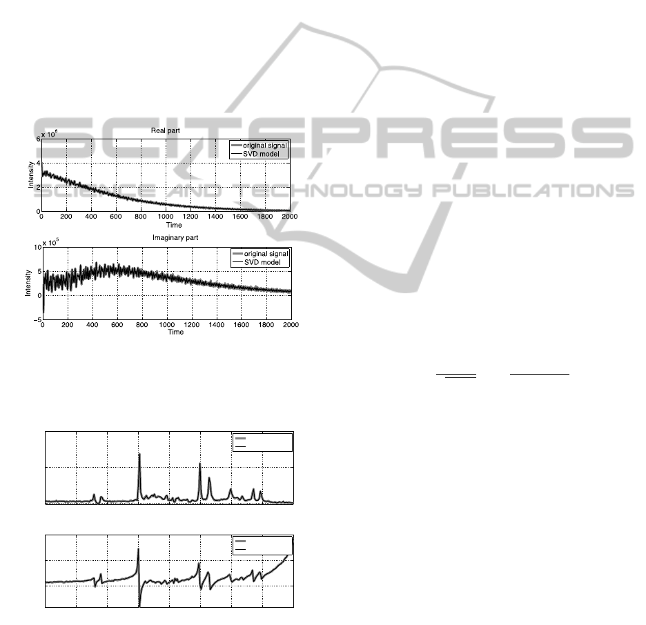
In figure 1 and figure 2 we present examples of
results of modelling the NMR signal by using
HSVD decomposition method. The number of
components K in (10) through (14) was set K=35.
This estimate was taken as equal to the number of
Gaussian components in the GMM method,
described in the next section, obtained by using the
Bayesian information criterion (BIC). In figure 1 we
show real and imaginary parts of the FID signal and
its HSVD model with K=35 components, while in
figure 2 we show real and imaginary parts of the
Fourier spectra of the FID signal and its HSVD
model.
Figure 1: FID signal for exemplary NMR data and its
HSVD model with K=35 components. Upper plot – real
part of the FID, lower plot – imaginary part of FID.
Colors: red, original signal- blue.
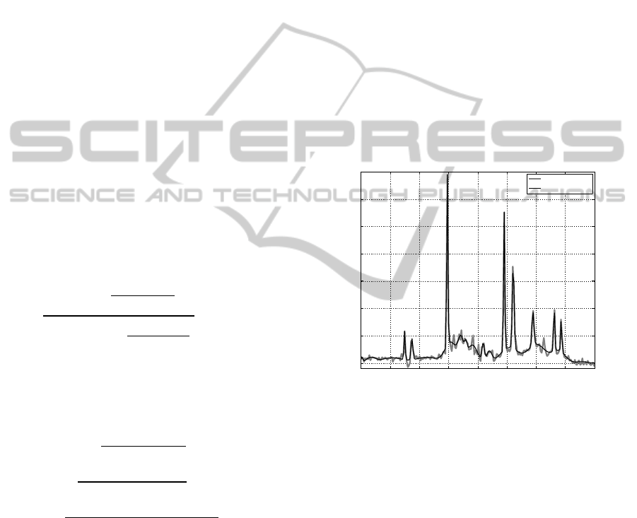
Figure 2: Fourier transforms (spectra) of a FID signal of
an exemplary NMR data and its HSVD model with K=35
components. Upper plot – real part of the spectrum, lower
plot – imaginary part of the spectrum. Colors: red, original
signal- blue.
3.2 Gaussian Mixture Model
The second black box approach for quantification of
NMR spectra involves modelling in the frequency
domain. The frequency domain analysis is based on
the application of the Fourier transform to the FID
signal (1). Quantitative information about metabolite
amount in tissue under investigation is done on the
basis of the real part of the frequency spectrum of
the FID signal (Gunther, 1992).
Since black box modelling assumes no prior
knowledge on the structure of the frequency
spectrum then the decomposition must be
performed, such that components will correspond to
hypothetical species present in the analysed tissue
(sample). The possible solution to the problem is to
use a mixture model (McLachlan and Peel, 2000),
where the amplitude spectrum corresponding to the
FID signal is represented as a sum of components
detected in the amplitude spectrum. Analytical
computations imply that damped sinusoidal signals
in the time domain correspond to Lorenzian
components in the frequency domain. However, due
to finite range of frequencies and due to existence of
the noise in the signal Gaussian mixture model
(GMM) can be a reasonable approximation for
amplitude spectrum of the FID signal (Jacobsen,
2007), GMM is constructed under the hypothesis
that there is K Gaussian components in the
amplitude spectrum. Each of these components is
represented by a Gaussian distribution function
described by a formula
,,
1
√
2
exp
2
(10)
and a mixture distribution composed of Gaussian
components (10) has the form:
,
,……,
,
,….,
,
,….,
,
,
(11)
In the above formulae (10) and (11) x denotes a data
point – a value of an amplitude of the frequency
spectrum,
and
are means and standard
deviations of mixture distribution functions and
are componentsweights. Component weights must
satisfy the normalization criterion
1.
(12)
The model (10)-(12) must be additionally scaled in
order to properly represent the amplitude spectrum
of the FID signal (Polanski and Kimmel, 2007)
.
0.5 1 1.5 2 2.5 3 3.5 4 4.5
0
5
10
PPM
Intensity
Real part
original signal
SVD model
0.5 1 1.5 2 2.5 3 3.5 4 4.5
0
5
10
PPM
Intensity
Imaginary part
original signal
SVD model
BIOSIGNALS2015-InternationalConferenceonBio-inspiredSystemsandSignalProcessing
60
For simplicity we drop superscript symbol and
absolute value operator and we formulate the scaled
mixture model as follows
,
,
(13)
In the above is a scale parameter and
is a
simplified notation for
.
A most commonly used computational iterative
algorithm for fitting GMM model parameters to data
is Expectation Maximization (EM) (Dempster,
1977). Due to application of the scaled form of the
mixture model appropriate formulation (variant) of
the EM algorithm is necessary, as described below.
EM for mixture parameters estimation relies on a
latent variable describing the hypothetical identity of
the component, which generated the observation x.
At the beginning a parameter guess is taken
,…,
,
,…,
,
,…,
.
(14)
Then two main steps of the iterations expectation (E)
and maximization (M) are alternately executed. In
the E step conditional probabilities for the latent
variable are calculated according to the formula (15)
(Polanski and Kimmel, 2007).
|
,
exp
∑
exp
(15)
In the M step the expectation of the logarithmic
likelihood function is maximized with respect to
parameters. This leads to the following updates of
parameter values
∑
|
,
∑
,
(16)
∑
|
,
∑
|
,
,
(17)
∑
|
,
∑
|
,
.
(18)
In order to efficiently use the EM algorithm with
given NMR spectroscopy data several further
adjustments are necessary (Binczyk et al., 2010).
1. Initial values of parameters are drawn
randomly. Mean values are drawn on the basis
of uniform sampling distribution defined by the
ranges of the frequency values. Component
weights from the Dirichlet distribution.
Component standard deviations are assumed
constant.
2. In order to better explore possible multiple
local maxima of the log likelihood function the
process of iterations is repeated for about 150
times, each with different guess for initial
values of mixture model components
parameters.
3. The number of components of the mixture K is
successively incremented and for each value
the Bayesian information criterion (BIC) is
calculated according formula
2ln
3
1 ln
∑
.
(19)
The number of components corresponding the
largest value of BIC obtained is chosen as the
estimate of the true value of K (Millar, 2006).
When computed for successive values of K, the
plot BIC versus K shows a minimum point, which
corresponds to estimate of the values fore each
mixture component. Exemplary mixture model
scaled to original signal is presented on the figure 3.
Figure 3: Real part of the frequency spectrum of the
exemplary NMR signal versus its GMM model with K=35
components. Colours: real part of the spectrum of the
original NMR signal – blue, GMM model of the spectrum
– red.
4 EXPERIMENT AND RESULTS
The data set used during experiments consists of
series of NMR spectra obtained for one phantom
data using NMR GE 1.5T Signal Echo Speed
scanner. The primary goal of scheduling the
experiment performed with the use of GE scanner
was to verify repeatability of the device for the same
data set. The series of experimental phantom
measurements was repeated each week through 4
months. The phantom sample contained metabolites:
12.5 mM of NAA, 10 mM of creatine, 3 mM of
choline (Cho), 7.5 mM of myo-inositol, 5 mM of
0.5 1 1.5 2 2.5 3 3.5 4 4.5
0
1
2
3
4
5
6
7
PPM
Intensity
original signal
GMM model
ComparisonofBlackBoxImplementationsofTwoAlgorithmsofProcessingofNMRSpectra,GaussianMixtureModel
andSingularValueDecomposition
61

lactate, 50 mM of potassium, 12.5 mM of sodium
hydroxide and 1ml/L of magnevist.
The original study measured in LC Model
consists of metabolite concentration and relation of
metabolites with respect to creatine. Authors for
further analysis used such ratios. For all of the data
sets were available measured water signals, which
were used in pre-processing techniques.
4.1 Comparisons of the Accuracy of
Modelling NMR Signals
Figure 4: Error of modelling NMR signal, calculated for
both methods: GMM (Y axis) and HSVD (X axis).
To compare ability of whole signal reconstruction,
results given by both methods: GMM and HSVD
were compared in interval 0.5-4.5 ppm. The overall
modelled signals were subtracted from original one
and error was calculated. The results are presented in
a form of scatter plot in which each point represents
an error calculated for a spectrum from set of 27 in a
coordination set spanned by error values for 2
modelling algorithms: HSVD on axis x and GMM
on axis y.
From above one can notice that there is
Pearson’s correlation equal to: 0,61, between result
of two proposed methods. It means that one of them
is slightly better from the other. To determine which
one is it basic statistics were calculated and shown in
Table 1.
Table 1: Mean value of error of overall signal modelling
and its 95 % CI calculated for both signal modelling
methods: HSVD and GMM.
Method Mean value of error
[Counts]
95 % CI
[Counts]
SVD
1.076 0.028
GMM
1.118 0.024
From above table it is easy to notice that HSVD
technique gives slightly better results in analysis of
whole signal (all possible peaks).
4.2 Comparisons of the Accuracy of
Estimation of Metabolite
Concentrations
Constructed GMM is then used to obtain
information about metabolite dispersion and amount
in tested specimen. To do so authors proposed to use
a convolution of chosen mixture model component
(or group of peaks- dependent on metabolite) and a
signal.
Each component of proposed model may be
understood as an independent peak from the
spectrum. Parameters of Gaussian component are
responsible for peak description: weight of
component- peak height, mean value of the
component- peak position in spectrum or frequency
and component variance – peak width. Authors
decided to use set of 27 spectra while for all of them
it was possible to use results obtained with use of
commercial solution LC Model developed by
Proventure (Provencher, 1993; Provencher, 1995).
Additionally data were analysed by Tarquin
software, which is free to use. All of obtained results
were compared with LC model reports. For such a
report it was possible to retrieve results for each
chosen metabolite and its relation with respect to
creatine. Results of all 4 algorithms (including LC
Model and Tarquin) were compared in means of
boxplots. Authors proposed to present recurrence of
results with use of relation true values. In order to
present them in clear and understandable way, the
results are shown on the separate plots for each
chosen metabolite by means of their main peak.
Authors did not have enough data to calculate
correction coefficient for transverse and longitude
relaxation. Therefore for comparison authors
decided to correct results with use of derived
coefficient of correction based on known value of
metabolite amount in the phantom. Such a
methodology implies division of the 27 spectra
dataset into two subsets: training and validating. The
training subject was decided to contain 12 spectra
and the others were used to verify estimated
correction coefficient.
0.95 1 1.05 1.1 1.15 1.2 1.25
0.95
1
1.05
1.1
1.15
1.2
1.25
HSVD
GMM
BIOSIGNALS2015-InternationalConferenceonBio-inspiredSystemsandSignalProcessing
62
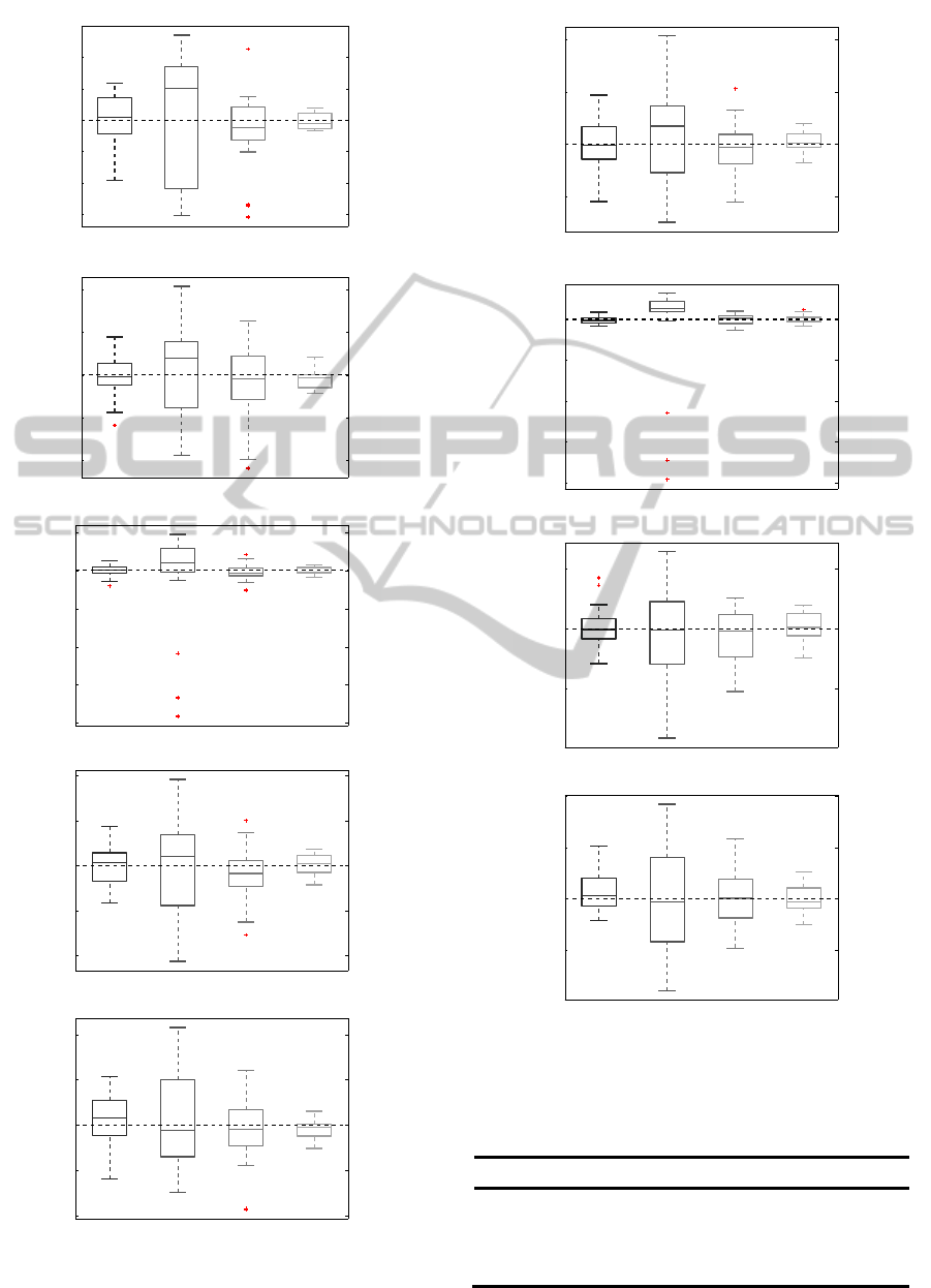
Figure 5: Comparison of 4 methods in terms of
concentration of metabolite.
Figure 6: Comparison of 4 methods in terms of relation to
Creatine.
Table 2: Comparison of Approximation error of
metabolites.
Relative error [%]
Creatine Naa Choline Lactate Inositol
LC
Model
1,940 2,760 2,167 3,440 2,960
Tarqu
in
4,290 6,872 11,533 8,940 5,400
HSVD
3,180 3,256 2,800 4,500 3,653
GMM
1,010 0,928 1,733 2,080 1,453
11
11.5
12
12.5
13
13.5
14
LCModel Tarquin HSVD GMM
Concentration [mM]
Naa
9
9.5
10
10.5
11
LCModel Tarquin HSVD GMM
Concentration [mM]
Creatine
1
1.5
2
2.5
3
3.5
LCModel Tarquin HSVD GMM
Concentration [mM]
Choline
4
4.5
5
5.5
6
LCModel Tarquin HSVD GMM
Concentration [mM]
Lactate
6.5
7
7.5
8
8.5
LCModel Tarquin HSVD GMM
Concentration [mM]
Inositol
1.2
1.25
1.3
1.35
LCModel Tarquin HSVD GMM
Relation to Creatine
Naa/Creatine
0.1
0.15
0.2
0.25
0.3
LCModel Tarquin HSVD GMM
Relation to Creatine
Choline/Creatine
0.45
0.5
0.55
LCModel Tarquin HSVD GMM
Relation to Creatine
Lactate/Creatine
0.7
0.75
0.8
0.85
LCModel Tarquin HSVD GMM
Relation to Creatine
Inositol/Creatine
ComparisonofBlackBoxImplementationsofTwoAlgorithmsofProcessingofNMRSpectra,GaussianMixtureModel
andSingularValueDecomposition
63

Table 2a: Comparison of Approximation error of relations.
Relative error [%]
Naa Choline Lactate Inositol
LC Model
1,360 1,333 2,600 2,000
Tarquin
3,120 11,000 5,600 5,867
HSVD
1,520 2,000 3,600 2,533
GMM
0,640 1,333 2,000 1,467
5 DISCUSSION AND
CONCLUSIONS
Data set that was used during experiments was
originally used to verify recurrence of newly bought
GE scanner. Such results were tested in each week
in few months time for the same phantom to check if
obtained results are comparable. For the comparison
authors took main peaks of 5 metabolites: Naa,
Creatine, Choline. Lactate, Myoinositol and checked
relations of metabolite with respect to Creatine (such
ratio is commonly used in oncology). The main idea
for this study was application of black box methods
without any additional prior knowledge. It was
decided to implement and compare two different
methods of signal analysis. One that is focused in
time domain analysis and on the other hand on
frequency domain. According to authors experience
and performed literature study there are few methods
basing on Singular Value Decomposition however
HSVD seems to be more accurate. In case of
frequency domain it was observed that peaks poses
Gaussian shape. It was then decided to use Gaussian
Mixture Model. Both methods were implemented in
Matlab-Simulink software as two separated tools for
NMR spectra analysis.
Authors decided to verify recurrence of obtained
results, which gave an answer for the question,
whether proposed methods could give reliable
results. Results obtained with use of two
implemented and tuned modelling methods were
compared to already existing solution - LC Model.
Results look reliable. After analysis of obtained
boxplots, authors may conclude that obtained
modelling algorithms are not worse than already
used- LC Model. What is more in some cases they
were even better. However HSVD technique gives
better results during analysis of whole signal with all
possible peaks. (Table 1)
First method applied to the phantom data was
method based on Gaussian mixture model. Authors
observed that in comparison to LC Model data,
which were treated as a reference values, its result is
satisfactory. It is so, because the aim of the method
is construction of a good fitted model of the data.
However authors observed that for some cases result
obtained by calculating the convolution of specific
Gaussian component and a signal differs from the
reference one. It might be caused by additional
components that are present in the data. Such a
components are: phase error, baseline and noise. The
study under consideration was a phantom
measurement so authors decided to neglect influence
of phase error and baseline. Signal noise is not only
visible as additional low amplitude peaks in
frequency spectrum, but also influences peak height.
In such a case peak and noise component are easily
recognized as just one component of mixture model.
To deal with the problem author’s decided to use
Savitzky-Golay approach while result was
satisfactory and the amplitude of filtered signal was
not damped. Such a filtering technique was applied
to the data in frequency domain- spectrum. It is
author’s suspicion that LC Model may use filters
that deal with FID instead of signal in frequency
domain. What is worth to notice, original idea of
GMM application to NMR spectroscopy data was to
analyse signals from many voxels instead of just
one. In such a case noise component that still
remains in the signal after application of Savitzky-
Golay [14] technique might be neglected. What is
more such an approach tells more about spatial
dependencies between metabolites instead of just
simple semi-quantification for each.
Methods based on SVD can be used in many pre-
processing techniques. Thanks to the fact that after
SVD decomposition singular values are arranged in
descending order one can notice that noise is present
always at the end of singular values. Such feature
can be applied in filtering of signal. Another
approach is connected to phase correction, which
relies on finding and correcting particular
component of FID. HSVD can model signal with
high precision depending on number of components
that is expected in result. In comparison to EM it
processes on FID in time domain and it strongly
depends on number of points that generates time
consumption. Many modifications of calculating
SVD have been proposed such as for example
Lanczos algorithm.
In order to calculate correct metabolites
concentration by means of SVD proper pre-
processing has to be done. In the next step method
should calculate components parameters and one
should identify metabolites that are searched and
build them from obtained components. The
concentration is based on calculating area under
peak present in spectrum by used of trapezoidal rule.
It has to be mentioned that before metabolites
BIOSIGNALS2015-InternationalConferenceonBio-inspiredSystemsandSignalProcessing
64

analysis optimal pre-processing has to be performed,
otherwise results may be incorrect.
As authors shown both of mentioned methods
gave satisfactory result, according to the reference
and what is more widely used software solution.
Taking into account all experiments performed by
authors it was proven that both methods might be
successfully used for analysis of NMR spectroscopy
data. Authors observed that crucial points is
sensitivity of both methods for unwanted
components such as noise that might not be
completely removed with advance techniques.
Authors decide to focus on improvement of that
crucial part in their future research.
ACKNOWLEDGMENTS
This work was financed by:
BKM515/2014/9 (MS), HARMONIA 4 register
number 2013/08/M/ST6/00924 (JP), BKM 524/Rau-
1/2014 (FB) and GeCONiI (POIG.02.03.01-24-
099/13) (AP).
All calculations were carried out using infrastructure
of GeCONiI (POIG.02.03.01-24-099/13).
REFERENCES
Beer R., Ormondt D., Pijnappel W.: Quantification of 1-D
and 2-D magnetic resonance time domain signals, Pure
&Appl. Chem., Vol. 64, No. 6, pp: 815-823, (1992).
Behar, K. L., Rothman, D. L., Spencer, D. D., Petroff,
O.A.:. Analysis of macromolecule resonances in 1H
NMR spectra of human brain. Magn. Reson. Med. 32
(3), 294–302, (1994).
Binczyk F. Tarnawski R. Polanska J: Mixture model of
NMR and its application to diagnosis and treatment of
brain cancer. Archives of Control Science 2010, 20(4),
pp:457-472, (2010).
Dempster A.: Maximum likelihood from in- complete data
via the EM algorithm. Journal of the Royal Statistical
Society B, 39(1), pp: 1-22 (1977).
McLachlan G., Peel D: Finite Mixture Models, ISBN:
047165406X, 9780471654063 Wiley & Sons (2000).
Graff R: In vivo NMR spectroscopy. Principles and
Techniques, Wiley & Sons, ISBN: 978-0-470-02670-0
(2007).
Gunther H.: NMR SPECTROSCOPY Basic Principles,
Concepts, and Applications in Chemistry, XIII-XIV,
241-243, ISBN: 978-0-471-95201- (1992).
Hofmann, L., Slotboom, J., Boesch, C., Kreis, R.,:
Characterization of the macromolecule baseline in
localized (1)H-MR spectra of human brain. Magn.
Reson. Med. 46 (5), 855–863 (2001).
Jacobsen N: NMR SPECTROSCOPY EXPLAINED
Simplified Theory, Applications and Examples for
Organic Chemistry and Structural Biology, 4-8, 118-
134, ISBN: 978-0-471-73096-5 (2007).
Krone M., Klawonn F., Luhrs T., Ritter C.: Identification
of Nuclear Magnetic Resonance Signals via Gaussian
Mixture Decomposition, Advances in Intelligent Data
Analysis X, Lecture Notes in Computer Science
Volume 7014, 2011, pp 234-245, (2011).
Lupu D., Todor D: A singular value decomposition based
algorithm for multicomponent exponential fitting of
NMR relaxation signals, Chemometrics and Intelligent
Laboratory Systems 29, pp: 11-17 (1995).
Millar P.: Using the Bayesian Information Criterion to
judge models and statistical significance”, North
American Stata Users' Group Meetings (2006).
Müller N.; Jerschow A. Nuclear Spin Noise Imaging.
Proc. Natl. Acad. Sci. U.S.A. 103, 6790–6792 (2006).
Savitzky A., Golay M.: Smoothing and differentiation of
data by Simplified least squares procedures. Analytical
Chemistry, 36(8), 1627-1639 (1964).
Polanski A., Kimmel M.: Bioinformatics. Springer-Verlag
New York, Inc., Secaucus, NJ, USA, ISBN: 978-
3540241669 pp: 43-45 (2007).
Provencher S.: Automated quantitation of localized
1
HNMR spectra in vivo: Capabilities and limitations.,
Proc SMR, 1952 (1995).
Provencher S.: Estimation of metabolite concentrations
from localized in vivo proton NMR spectra. Magn.
Reson. Med.; 30: 672–679, (1993).
Weinreb, J. C., Brateman, L., Babcock, E. E., Maravilla,
K.R., Cohen, J.M., Horner, S.D.,: Chemical shift
artifact in clinical magnetic resonance images at 0.35
T. AJR Am. J. Roentgenol. 145 (1), 183–185, (1985).
Wilson, M., Reynolds, G., Kauppinen R. A., Arvanitis T.
N., Peet A. C.: A constrained least-squares approach to
the automated quantitation of in vivo 1H magnetic
resonance spectroscopy data. Magn. Reson. Med. 65
(1), 1–12, (2010).
ComparisonofBlackBoxImplementationsofTwoAlgorithmsofProcessingofNMRSpectra,GaussianMixtureModel
andSingularValueDecomposition
65
