Machine Reading of Biological Texts

Bacteria-Biotope Extraction

Wouter Massa

, Parisa Kordjamshidi

1,2

, Thomas Provoost

and Marie-Francine Moens

Department of Computer Science, KU Leuven, Celestijnenlaan 200A, 3001, Heverlee, Belgium

Department of Computer Science, University of Illinois at Urbana-Champaign,

201 North Goodwin Avenue, 61801-2302, Urbana, IL, U.S.A.

Keywords:

Natural Language Processing, Text Mining, Relation Extraction, BioNLP, Bioinformatics, Bacteria, Bacteria

Biotopes.

Abstract:

The tremendous amount of scientiﬁc literature available about bacteria and their biotopes underlines the need

for efﬁcient mechanisms to automatically extract this information. This paper presents a system to extract

the bacteria and their habitats, as well as the relations between them. We investigate to what extent current

techniques are suited for this task and test a variety of models in this regard. To detect entities in a biological

text we use a linear chain Conditional Random Field (CRF). For the prediction of relations between the entities,

a model based on logistic regression is built. Designing a system upon these techniques, we explore several

improvements for both the generation and selection of good candidates. One contribution to this lies in the

extended ﬂexibility of our ontology mapper, allowing for a more advanced boundary detection. Furthermore,

we discover value in the combination of several distinct candidate generation rules. Using these techniques,

we show results that are signiﬁcantly improving upon the state of art for the BioNLP Bacteria Biotopes task.

1 INTRODUCTION

A vast amount of scientiﬁc literature is available about

bacteria biotopes and their properties (Bossy et al.,

2013). Processing this literature can be very time-

consuming for biologists, as efﬁcient mechanisms

to automatically extract information from these texts

are still limited. Biologists need information about

ecosystems where certain bacteria live in. Hence,

having methods that rapidly summarize texts and list

properties and relations of bacteria in a formal way

becomes a necessity. Automatic normalization of the

bacteria and biotope mentions in the text against cer-

tain ontologies facilitates extending the information in

ontologies and databases of bacteria. Biologists can

then easily query for speciﬁc properties or relations,

e.g. which bacteria live in the gut of a human or in

which habitat Biﬁdobacterium Longum lives.

The Bacteria Biotopes subtask (BB-Task) of the

BioNLP Shared Task (ST) 2013 is the basis of this

study. It is the third event in this series, following the

same general outline and goals of the previous events

edellec et al., 2013). BioNLP-ST 2013 featured six

event extraction tasks all related to “Knowledge base

construction”. It attracted wide attention, as a total of

38 submissions from 22 teams were received.

The BB-Task consists of three subtasks. In the

ﬁrst subtask habitat entities need to be detected in a

given biological text and the entities must be mapped

onto a given ontology. The habitat entities vary from

very speciﬁc concepts like ‘formula fed infants’ to

very general concepts like ‘human’. The second sub-

task is focused on the extraction of two relations: a

Localization and a PartOf relation. These relations

need to be predicted between a given set of entities

(bacteria, habitats and geographical locations). Lo-

calization relations occur between a bacterium and

a habitat or geographical location, PartOf relations

only occur between habitats. The third subtask is an

extended combination of the two other subtasks: enti-

ties need to be detected in a text and relations between

these entities need to be extracted. In this paper we fo-

cus on the ﬁrst two subtasks.

We ﬁrst describe related work done in context of

the BioNLP-ST (Section 2). We then discuss our

methodology for the two subtasks (Section 3). Next,

we discuss our experiments and compare our results

with the ofﬁcial submissions to BioNLP-ST 2013

(Section 4). We end with a conclusion (Section 5).

Massa W., Kordjamshidi P., Provoost T. and Moens M..

Machine Reading of Biological Texts - Bacteria-Biotope Extraction.

DOI: 10.5220/0005214700550064

In Proceedings of the International Conference on Bioinformatics Models, Methods and Algorithms (BIOINFORMATICS-2015), pages 55-64

ISBN: 978-989-758-070-3

 2015 SCITEPRESS (Science and Technology Publications, Lda.)

2 RELATED WORK

The BB-task along with the experimental dataset has

been initiated for the ﬁrst time in the BioNLP Shared

Task 2011 (Bossy et al., 2011). Three systems were

developed in 2011 and ﬁve systems for its extended

version proposed in the 2013 shared task (Bossy et al.,

2013). In 2011 the following systems participated in

this task. TEES (Bjorne and Salakoski, 2011) was

proposed by UTurku as a generic system which uses

a multi-class Support Vector Machine classiﬁer with

linear kernel. It made use of Named Entity Recogni-

tion patterns and external resources for the BB model.

The second system was JAIST (Nguyen and Tsu-

ruoka, 2011), speciﬁcally designed for the BB-task.

It uses CRFs for entity recognition and typing and

classiﬁers for coreference resolution and event extrac-

tion. The third system was Bibliome (Ratkovic et al.,

2011), also speciﬁcally designed for this task. This

system is rule-based, and exploits patterns and do-

main lexical resources.

The three systems used different resources for

Bacteria name detection which are the List of

Prokaryotic Names with Standing in Nomenclature

(LPNSN), names in the genomic BLAST page of

NCBI and the NCBI Taxonomy, respectively. The

Bibliome system was the winner for detecting the

Bacteria names as well as for the coreference reso-

lution and event extraction. The important factor in

their outperformance was exploiting the resources and

ontologies. They found useful matching patterns for

the detection of entities, types and events. Using their

manually drawn patterns and rules performed better

than other task participant systems, in which learning

models apply more general features.

In the 2013 edition of this task, the event extrac-

tion is deﬁned in a similar way but an extension to

the 2011 edition considered biotope normalization us-

ing a large ontology of biotopes called OntoBiotope.

The task was proposed in three subtasks to which we

pointed in Section 1. Five teams participated in these

subtasks. In the ﬁrst subtask all entities have to be

predicted, even if they are not involved in any rela-

tion. The participated systems performed reasonably

well. However, the difﬁculty of this task has been

boundary detection.

The participating systems obtained a very low re-

call for the relation extraction even when the entities

and their boundaries are given (subtask 2 and 3). The

difﬁculty of the relation extraction is partially due to

the high diversity of bacteria and locations. The many

mentions of different bacteria and localization in the

same paragraph makes it difﬁcult to select the right

links between them. The second difﬁculty lies in the

high frequency of anaphora. This makes the extrac-

tion of the relations beyond sentence level difﬁcult.

The strict results of the third task were very poor,

due to struggling with the difﬁculties of both previ-

ous tasks i.e, boundary detection and link extraction.

For detecting entities (subtask 1), one submission

(Bannour et al., 2013) worked with generated syntac-

tical rules. Three other submissions (Claveau, 2013),

(Karadeniz and

Ozg

ur, 2013) and (Grouin, 2013) used

an approach similar to ours. They generated candi-

dates in an initial phase from texts. These candidates

were subsequently selected by trying to map them

onto the ontology. Two submissions (Claveau, 2013)

and (Karadeniz and

Ozg

ur, 2013) generated candi-

dates by extracting noun phrases. One submission

(Grouin, 2013) used a CRF model to generate candi-

dates, as we do in this work. However, we test candi-

dates more thoroughly and consider every continuous

subspan of tokens in each candidate instead of just the

candidate itself, which explains our improved results.

For the relation extraction with given entities (sub-

task 2), there were four submissions. One system

from LIMSI (Grouin, 2013) relied solely on the fact

that the relation was seen in the training set which

fails to yield a reasonable accuracy. A second sys-

tem BOUN (Karadeniz and

Ozg

ur, 2013) extracted

relations using only simple rules, e.g. in a speciﬁc

paragraph they created relations between all locations

and the ﬁrst bacterium in that paragraph. A third sys-

tem IRISA (Claveau, 2013) used a nearest neighbor

approach. Another system was TEES (Bj

orne and

Salakoski, 2013) (an improved version of the UTurku

participation in 2011) which provided the best results.

However, the results were still poor.

One reason for this lies in the limited scope of

candidates that the submitted systems considered,

e.g. TEES (Bj

orne and Salakoski, 2013) and IRISA

(Claveau, 2013) only examined relations between a

habitat and location that occur in the same sentence.

One of our contributions lies in considering more pos-

sible relations, including relations across sentences.

This is conﬁrmed by a much better recall, as can be

seen in Section 4.3.2.

3 METHODOLOGY

In this section we lay out our developed system. For

each of subtasks 1 and 2, we ﬁrst discuss the goal of

the subtask, followed by an explanation of our used

methodology. The performance of our model is dis-

cussed in the next section (Section 4).

BIOINFORMATICS2015-InternationalConferenceonBioinformaticsModels,MethodsandAlgorithms

3.1 Subtask 1: Entity Detection and

Ontology Mapping

The goal of this subtask is to detect habitat entities

in texts and map them onto concepts deﬁned by the

OntoBiotope-Habitat ontology. For each entity the

name, the location in the text and the corresponding

ontology entry need to be predicted. E.g. the ex-

pected output for a text consisting of the single sen-

tence “This organism is found in adult humans and

formula fed infants as a normal component of gut

ﬂora.” is:

T1 Habitat 27 33 adult humans

T2 Habitat 44 63 formula fed infants

T3 Habitat 44 51 formula

T4 Habitat 89 92 gut

N1 OntoBiotope Annotation:T1 Ref:MBTO:00001522

N2 OntoBiotope Annotation:T2 Ref:MBTO:00000308

N3 OntoBiotope Annotation:T3 Ref:MBTO:00000798

N4 OntoBiotope Annotation:T4 Ref:MBTO:00001828

Four habitat entities are found in this sentence and

they are mapped onto four different ontology entries.

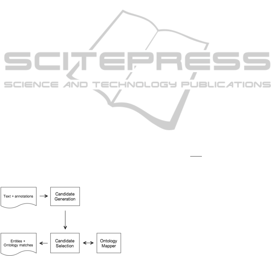
Figure 1 gives an overview of the followed ap-

proach. We ﬁrst search in the text for token spans

(candidates) that might contain one or more enti-

ties (Section 3.1.1). These generated candidates are

given to a Candidate Selection module, that searches

substrings within the candidate for entities (Section

3.1.3). This Candidate Selection module uses an On-

tology Mapper (Section 3.1.2), ﬁnding the ontology

entry that matches closest to a given substring. Ad-

ditionally it returns a dissimilarity value to give an

indication of how close the match is. Based on this

dissimilarity, we can decide to classify part of a can-

didate as the given entry or not.

Figure 1: Overview of the followed approach in subtask 1.

3.1.1 Candidate Generation

The Candidate Generation module generates token

spans from a given input text. The goal of the Gener-

ation module is to quickly reduce a large text to a can-

didate set that can be analysed more efﬁciently. First

the text is split into sentences and tokens, then ev-

ery sentence is mapped onto a set of candidates. We

use the given annotation ﬁles of the Stanford Parser

(Klein and Manning, 2003) to split the texts and to-

kenize the sentences. Sentences are assumed to be

independent in the model, i.e. we do not use informa-

tion from one sentence in another sentence.

Conditional Random Fields. To generate candi-

dates, we use Conditional Random Fields (CRF) (Sut-

ton and McCallum, 2006). In particular, we choose a

linear chain CRF; previous research shows that these

perform well for various natural language process-

ing tasks, especially Named Entity Recognition (Lei

et al., 2014). In contrast to general purpose noun

phrase extractors used by some other existing models

for this task, a CRF can easily exploit the information

of the given annotated ﬁles as features.

A CRF model is an undirected probabilistic graph-

ical model G = (V, E) with vertices V and edges E.

The vertices represent a set of random variables with

the edges showing the dependencies between them.

The set of observed random variables is denoted by

X and the unknown/output random variables are de-

noted by Y . This model represents a probability dis-

tribution over a large number of random variables by a

product of local functions that each depend on a small

subset of variables, called factors.

A CRF generally deﬁnes a probability distribution

p(y|x), where x, y are speciﬁc assignments of respec-

tive variables X and Y as follows:

p(y|x) =

Z(x)

∏

∈G

, y

) (1)

where x

are those observed variables that are part of

factor F and similarly for y

and Y . Ψ

: V

→ R is

the potential function associated with factor F and is

deﬁned in terms of the features f

, y

) as:

, y

) = exp

(

∑

, y

)

(2)

The parameters of the conditional distribution λ

are

trained with labelled examples. Afterwards, using the

trained model the most probable output variables can

be calculated for a given set of observed variables.

Z(x) is a normalization constant and is computed as:

Z(x) =

∑

∏

∈G

, y

) (3)

CRFs can represent any kind of dependencies, but

the most commonly used model, particularly in the

NLP tasks such as Named Entity Recognition is the

Linear-chain model. In this work, we use the linear

chain implementation in Factorie (McCallum et al.,

MachineReadingofBiologicalTexts-Bacteria-BiotopeExtraction

2009). Linear chain CRFs consider the dependency

between the labels of the adjacent words. In other

words, each local function f

, y

t−1

, x

) represents

the dependency of each output variable y

in location

t in the chain to its previous output variable y

t−1

and

the observed variable x

at that location. The global

conditional probability then is computed as the prod-

uct of these local functions (Sutton and McCallum,

2006). With the usual assumption that all local func-

tions share parameters and feature functions, its log-

linear form is now written as:

p(y|x) =

Z(x)

exp

(

∑

, y

t−1

, x

)

(4)

Where the normalization constant is derived in an

analogous manner to equation (3) for the case of se-

quential dependencies.

In our model, every token is an observed variable. The

biological entity labels (e.g. ‘Bacterium’) of the to-

kens are the output variables (or labels).

We now discuss the features that we use, along

with the label set into which the tokens are classiﬁed.

CRF Features. The following features are used for

each token:

• Token string

• Stem

• Length token

• Is capitalized (binary)

• Token is present in the ontology (binary)

• Stem is present in the ontology (binary)

• Category of the token in the Cocoa annotations

• Part-of-speech tag

• Dependency relation to the head of the token

The stem is calculated using an online available

Scala implementation

of Porter’s stemming algo-

rithm (Porter, 1980). The part-of-speech tag and the

dependency relation to the head are added using the

available annotation ﬁles from the Stanford Parser

(Klein and Manning, 2003). Cocoa

is a dense anno-

tator for biological text. The Cocoa annotations cover

over 20 different semantic categories like ‘Processes’

and ‘Organisms’.

CRF Labels: Extended Boundary Detection Tags.

We use ﬁve different labels for the tokens. The used

labels are:

• Start: The token is the ﬁrst token of an entity.

https://github.com/aztek/porterstemmer

http://npjoint.com

• Center: The token is in the middle of an entity.

• End: The token is the last token of an entity.

• Whole: The token itself is an entity.

• None: The token does not belong to an entity.

The most immediate alternative to this is the tra-

ditional IOB labeling (Ramshaw and Marcus, 1995).

An even more simple possibility is a binary labeling

that just indicates if a token belongs to an entity men-

tion or not. The more elaborated proposed labeling

generally performs better in our tests.

3.1.2 Ontology Mapper

The Ontology Mapper maps a string onto the ontol-

ogy entry with the lowest dissimilarity. The dissim-

ilarity between an ontology entry and string is cal-

culated by comparing the string with the name, syn-

onyms and plural of the name and synonyms of the

entry with respect to a certain comparison function.

The plurals are calculated simply by just adding ‘s’ or

‘es’ to the end of the singular form.

To compare two strings they are split into tokens.

The tokens from the two strings are matched to mini-

mize the sum of the relative edit distance between the

matched tokens. If not all tokens can be matched i.e.

the number of tokens in the two strings are different,

1.0 is added to the sum for each remaining token. As

a measure for relative edit distance, we use the Lev-

enshtein distance (Levenshtein, 1966) divided by the

sum of the lengths of the strings to get a number be-

tween 0.0 and 1.0.

3.1.3 Candidate Selection

The Candidate Selection module receives spans of to-

kens as input, it searches within these spans for on-

tology entries. For each span every continuous sub-

span of tokens is tested with the Ontology Mapper.

This means that we select

n(n+1)

subspans for every

token span with n tokens. If for a subspan a dissimi-

larity lower than a speciﬁc bound is reached, we clas-

sify this subspan as an entity. E.g. for the token span

‘formula fed infants’, six subspans are selected: ‘for-

mula’, ‘fed’, ‘infants’, ‘formula fed’, ‘fed infants’ and

‘formula fed infants’. ‘formula’ and ‘formula fed in-

fants’ are found in the ontology and we classify these

as entities.

Based on cross-validation experiments on the

training and development set, we decided to take as

maximal dissimilarity 0.1, i.e. the subspan must be

very close to an ontology entry. This very strict pa-

rameter allows us to be less strict in the Candidate

Generation module: every entity that has a minimum

BIOINFORMATICS2015-InternationalConferenceonBioinformaticsModels,MethodsandAlgorithms

probability of 0.1 to contain entities will be tested.

The sensitivity of our results with respect to this mea-

sure is further discussed in Subsection 4.3.1 and Table

3.1.4 Additional Improvements

Dashed Words. Not all entities in the texts consist

of one or more tokens, some entities are only a part of

a token. E.g. in the token ‘tick-born’, ‘tick’ is an en-

tity. To handle these cases we search for all the words

that contain one or more dashes. These words are split

and every part is matched against the ontology. These

parts are easy to match because they are usually just

nouns in singular form.

Extending the Ontology. Mappings from phrases

onto ontology entries are given in the training and de-

velopment set. These phrases are usually similar to

the name or a synonym of the ontology entry. How-

ever in rare cases the phrase is not similar to the name

or a synonym. Based on the assumption that the given

mapping is correct we can extend the ontology. We do

this by adding the phrase as a new synonym to the on-

tology entry. Some submissions to the BioNLP-ST

2013 task used this approach as well (Grouin, 2013),

(Karadeniz and

Ozg

ur, 2013).

Correcting Boundaries. An important part of the

task is to predict the correct boundaries of the enti-

ties. E.g. for the noun phrase ‘blood-sucking tsetse

ﬂy’, it is not sufﬁcient to predict ‘ﬂy’ or ‘tsetse ﬂy’.

The whole noun phrase is the correct entity in this

case. This particular example is hard because ‘blood-

sucking tsetse ﬂy’ does not occur in the ontology. To

handle this case we add to each found entity the de-

pendent words that precede the entity. These depen-

dent words can be extracted by using the given parser

annotations. E.g. from the phrase ‘blood-sucking

tsetse ﬂy’ the entity ‘tsetse ﬂy’ is selected, ‘blood-

sucking’ is added to it because its headword is ‘ﬂy’.

Filter out Parents. Many generated candidates re-

fer to the same entity, it is required that we predict

every entity only once. E.g. in the phrase ‘person

with untreated TB’ the entities ‘person’ and ‘person

with untreated TB’ are detected. They refer both to

the same habitat, ‘person’ is just a more general term

to describe ‘person with untreated TB’. That is why

we ﬁlter ‘person’ out. We can do this by using the

parent/child relations given in the ontology. The on-

tology entry ‘person’ is a parent (a more general term)

of the entry ‘person with untreated TB’, so we only

predict the phrase ‘person with untreated TB’ in this

case. Because the ontology is a deep graph of entities,

we test this parent/child relationship recursively.

3.2 Subtask 2: Relation Extraction

In this subtask relations need to be extracted from a

text based on annotated entities in the text. There are

three types of entities: habitats, geographical entities

and bacteria. Two types of relations exists: Local-

ization and PartOf. Localization relations are always

between a bacterium and a habitat or geographical lo-

cation. PartOf relations occur between two habitats.

We handle these two relations independently. In the

training and development set combined, Localization

and PartOf relations are responsible for respectively

81% and 19% of the relations.

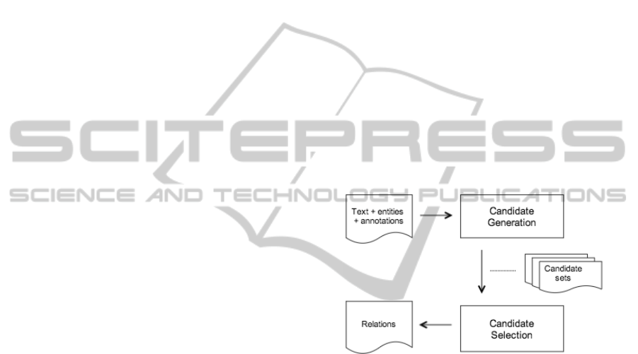
We used a similar approach for both relation types.

We will describe our approach for Localization rela-

tions. Our model consists of two modules. A ﬁrst

module generates sets of relation candidates from the

text using simple rules (Section 3.2.1). These sets are

then forwarded to a second module that trains for each

set a separate model (Section 3.2.2). Figure 2 shows

a visualization of our approach.

Figure 2: Overview of the followed approach in subtask 2.

3.2.1 Candidate Generation

The Candidate Generation module reduces the set of

all possible relations, i.e. all combinations of bacte-

ria and locations, to multiple smaller sets of candidate

relations. Every set is created by using a generation

rule. These smaller sets are then forwarded to the

Candidate Selection module that will try to identify

if a candidate relation is really a relation or not.

We use generation rules for two reasons. On one

side we decrease the overall number of candidates by

a signiﬁcant amount. On the other side we group sim-

ilar types of relations to build more speciﬁc models.

For every set of candidate relations deﬁned by a gen-

eration rule, we build a separate model to test these

relations. A good candidate generation method gen-

erates a relatively large number of correct relations

while keeping the number of wrong relations to a min-

imum.

We tested 5 different candidate generation rules

for Localization relations:

MachineReadingofBiologicalTexts-Bacteria-BiotopeExtraction

• All Possible: All combinations of bacteria and lo-

cations are possible.

• Same Sentence: The bacterium and location oc-

cur in the same sentence. This assumption is

used by two submissions: (Bj

orne and Salakoski,

2013) and (Claveau, 2013).

• Previous Bacteria: The bacterium is the ﬁrst bac-

terium that occurs before the location in the text.

• Next Bacteria: The bacterium is the ﬁrst bac-

terium that occurs after the location in the text.

• Paragraph Subject: The text is split into para-

graphs. The bacterium is the ﬁrst bacterium that

occurs in the paragraph of the location. This is

used by one submission: (Karadeniz and

Ozg

ur,

2013).

The results from section 4.3.2 are achieved by

combining the ‘Same sentence’ and ‘Previous bac-

teria’ generation rule, which yields the best perfor-

mance.

3.2.2 Candidate Selection

The Candidate Generation module forwards different

sets of candidate relations to the Candidate Selection

module. This Candidate Selection module builds for

every set a separate logistic regression model (using

the Factorie toolkit (McCallum et al., 2009)). We use

these logistic regression models as binary classiﬁers

(is a relation or not). In the training phase, the models

are trained based on positive and negative relations

extracted from example texts. In the testing phase,

each set of candidate relations is tested by their sepa-

rate model.

The model uses the following features based on

the two involved entities in a relation:

• The type of the entity

• Surface form

• Is capitalized (binary)

• Stem of each entity token

• Category of each entity token in the Cocoa anno-

tations

• Part-of-speech tag of each entity token

• Dependency relation to the head of each token

None of the above features combine information

from both the bacterium and location. We tested some

features that do this, but without a signiﬁcant inﬂu-

ence on F1, as we saw a slightly better precision with

a small drop in recall. The tested features are:

• Token distance between bacterium and location

• Length of syntactic path between bacterium and

location

• The depth of the tree that contains the syntactic

path

• Whether the bacterium or location occurs ﬁrst

Alternative Models. Besides this model we also

tested a nearest neighbor model. In this, we compare a

candidate with a seen example based on the sequence

of part-of-speech tags that occur on the syntactic path

between the bacterium and location. Between these

two sequences of tags the edit distance is calculated.

Finally, the candidate is classiﬁed as a relation if the

closest seen example with respect to this distance en-

codes a real relation.

In another approach we used two language models

based on the tokens between the bacterium and loca-

tion, where a separate model for positive and negative

relations was built. Here, a candidate is classiﬁed as

a relation if the probability that the candidate is gen-

erated by the positive model is higher than the proba-

bility for the negative model.

Both alternative models failed to achieve reason-

able performance.

4 EXPERIMENTS

In the ﬁrst subsection we describe the data set and the

resources. The subsections thereafter then present the

results and discussions.

4.1 Data Set

The data set consists of public available documents

from web pages from bacteria sequencing projects

and from the MicrobeWiki encyclopedia (Bossy et al.,

2013). The data is divided into a training, a develop-

ment and a test set. The solution ﬁles of the training

and development set are provided. The solution ﬁles

of the test set are not available, but it is possible to

test a solution with an online evaluation service

with

a minimal time of 15 minutes between two submis-

sions. During the contest the minimal time between

two submissions has been 24 hours. We limited our

use of the online evaluation service to keep our results

comparable with the contest submissions.

The data consists of 5,183 annotated entities and

2,260 annotated relations. The data was manually an-

notated twice followed by a conﬂict resolution phase

http://genome.jouy.inra.fr/∼rbossy/cgi-bin/bionlp-eval

/BB.cgi

BIOINFORMATICS2015-InternationalConferenceonBioinformaticsModels,MethodsandAlgorithms

(Bossy et al., 2013). Table 1 gives an overview of the

data distribution. The training and development set is

the same for both subtasks, but the test set is different.

Table 1: Summary statistics of the data set.

Training/Dev Testset 1 Testset 2

Documents 78 27 26

Words 25,828 7,670 10,353

Entities 3,060 877 1,246

Relations 1,265 328 667

4.2 Used Ontology

In the ﬁrst subtask the OntoBiotope-Habitat ontol-

ogy

is used. This ontology contains 1,756 habitat

concepts. For each concept an id, the name and ex-

act and related synonyms are given. Additionally if a

concept can be described by a more general concept,

an is a relation is given. The ontology entry ‘dental

caries’ is for example:

id: MBTO:00001830

name: dental caries

related_synonym: "tooth decay" [TyDI:30379]

exact_synonym: "dental cavity" [TyDI:30380]

is_a: MBTO:00002063 ! caries

4.3 Results

The results are presented separately for the two sub-

tasks of entity detection and relation extraction.

4.3.1 Entity Detection and Ontology Mapping

The score is calculated by mapping the predicted enti-

ties onto the entities of the reference solution. Entities

are paired in a way that the sum of the dissimilarities

are minimized. The dissimilarity between a predicted

entity and a reference entity is based on boundary ac-

curacy and the semantic similarity between the ontol-

ogy concepts. Based on this optimal mapping of enti-

ties the Slot Error Rate (SER) is calculated. A perfect

solution has a SER score of 0, if no entities are pre-

dicted a score of 1 is obtained. The SER is calculated

as follows:

SER =

S + I + D

(5)

• S: number of substitutions, based on the dissimi-

larity between the matched entities.

• I: number of insertions, the number of predicted

entities that could not be paired.

http://bibliome.jouy.inra.fr/MEM-OntoBiotope/Onto

Biotope BioNLP-ST13.obo

• D: number of deletions, the number of reference

entities that could not be paired.

• N: number of entities in the reference solution.

Improvement Effects. We implemented four vari-

ations to improve our model (see Section 3.1.4). The

highest improvement is achieved by correcting the

boundaries and ﬁltering out redundant parents. Al-

though handling dashed words gives only a slight im-

provement, it is deﬁnitely worth to use it because it

increases the number of found entities without creat-

ing much incorrect entities. Extending the ontology

improves our solution only by a very small margin.

Inﬂuence of the Maximal Dissimilarity. As ex-

plained in section 3.1.3, the Candidate Selection mod-

ule receives spans of tokens as input and searches

within these spans for ontology entries. For a spe-

ciﬁc subspan of tokens, the Ontology Mapper returns

the ontology entry that best matches, together with a

dissimilarity measure. Based on cross-validation ex-

periments we picked 0.1 as maximal dissimilarity, i.e.

we classify all subspans with a lower dissimilarity as

0.1 as a found entity.

Table 2 shows the SER score together with the

number of Substitutions, Insertions and Deletions (us-

ing 10 fold cross validation on the training and devel-

opment set) for several values of maximal dissimilar-

ity. For a range of low thresholds, only a very small

variation in the number of Substitutions and Deletions

is observed. However, the number of Insertions in-

creases steadily with an increasing maximal dissimi-

larity. This is because we allow subspans to be less

and less similar to the ontology entries, causing an in-

creasing number of wrongly extracted entities.

Table 2: Inﬂuence of the maximal dissimilarity on entity

detection performance.

Dissimilarity Sub Ins Del SER

0.05 212 195 181 0.38

0.10 210 197 180 0.38

0.15 212 208 180 0.39

0.20 211 212 180 0.39

0.25 227 236 173 0.41

0.30 230 249 169 0.41

0.35 319 497 141 0.61

Comparison with Contest Submissions. Testing

our model with the online evaluation service, we ob-

tained a SER score of 0.36 which is signiﬁcantly bet-

ter than all submissions to BioNLP-ST 2013. The best

result of the contest is a SER score of 0.46 (IRISA).

MachineReadingofBiologicalTexts-Bacteria-BiotopeExtraction

We also improved the precision and F1 compared

to all submissions. Recall, precision and F1 were re-

spectively 0.68, 0.73 and 0.70. The IRISA submission

scored a higher recall but a lower precision than our

model. Table 3 shows our scores together with the

scores of the submissions to BioNLP-ST 2013.

Table 3: Subtask 1 results compared to contest submissions.

Participant SER Recall Precision F1

IRISA 0.46 0.72 0.48 0.57

Boun 0.48 0.60 0.59 0.59

LIPN 0.49 0.61 0.61 0.61

LIMSI 0.66 0.35 0.62 0.44

Ours 0.36 0.68 0.73 0.70

Some reasons why we outperform the others are:

• With a CRF model it is easy to consider any infor-

mation through the addition of features. However,

many systems that use a CRF to generate candi-

dates are based on a general purpose noun phrase

extractor, and do not use the biological annota-

tions that are supplied.

• We search within each candidate for matches,

which makes it possible that a candidate contains

multiple entities.

• We redeﬁne the boundaries of an entity by us-

ing the head annotations from the given Stanford

parser annotated data.

The main weakness of our model is that an entity

needs to be very close to a name or synonym of an

ontology entry to be detected. We picked a value of

0.1 as maximal dissimilarity. This means that entities

that do not occur in the ontology or are described by

an unknown synonym can not be found. We imple-

mented an improvement by correcting the boundaries

to lower the impact of this weakness. In this way,

words that are not seen in the ontology can be part of

an entity if its head word occurs in the ontology.

4.3.2 Relation Extraction

Baseline Model. To better analyse the performance

of our approach, we have ﬁrst built a baseline model.

This model predicts Localization relations between

all bacteria and locations that occur in the same sen-

tence and no PartOf relations. The results are pre-

sented in Table 5. Considering the achieved scores in

BioNLP-ST 2013, this model performs dramatically

better. It outperforms all submissions based on F1

due to a much higher recall. But the precision of one

submission (TEES) is clearly better (0.82).

This baseline model predicts 53% of the Local-

ization relations. Based on the fact that this baseline

model only predicts relations within the same sen-

tence, we know that about half of the Localization re-

lations occur in the same sentence, for the other half

multiple sentences need to be examined.

Performance on Different Relation Types. We

use a similar approach for PartOf relations as for Lo-

calization relations. Table 4 shows the performance

of our model for the prediction of one relation type

separately and the prediction of both types jointly. We

see a very low precision if we only predict PartOf re-

lations, this is due to the fact that we recall many re-

lations wrongly and there are only few true PartOf

relations in the texts. When we combine our Local-

ization and PartOf model the result is worse than the

Localization model on itself. The PartOf model de-

creases the overall precision of our model much more

compared to the gain in recall.

Table 4: Relation extraction results for the different relation

types.

Model Recall Precision F1

Localization 0.59 0.50 0.54

PartOf 0.09 0.15 0.12

Combined 0.68 0.35 0.46

Comparison with Contest Submissions. We

tested our solution with the available online eval-

uation service and receive a F1 of 0.67 which is

signiﬁcantly better than all submissions to BioNLP-

ST 2013. The best result of the contest achieved

a F1 of 0.42 (TEES). Our recall and precision are

respectively 0.71 and 0.63. This recall is much higher

than all the contest submissions, one submission

(TEES) scored a better precision (0.82). Table 5

shows our achieved results together with the scores

of the ofﬁcial submissions to BioNLP-ST 2013.

Table 5: Subtask 2 results compared to contest submissions.

Participant Recall Precision F1

TEES-2.1 0.28 0.82 0.42

IRISA 0.36 0.46 0.40

Boun 0.21 0.38 0.27

LIMSI 0.04 0.19 0.06

Baseline 0.43 0.47 0.45

Ours 0.71 0.63 0.67

Some reasons why we outperform the others are:

• We use a combination of generation rules, the

contest submissions were mainly limited to one

speciﬁc generation rule.

• We do not predict PartOf relations in our ﬁnal

model due to low accuracy and overall negative

impact.

BIOINFORMATICS2015-InternationalConferenceonBioinformaticsModels,MethodsandAlgorithms

Bacterium Model. The logistic regression model

achieves signiﬁcantly better results than the baseline

model and all contest submissions. However, many

of the used features have only very little inﬂuence.

We remark that almost comparable results can be

achieved by a model that always predicts true unless

the bacterium name starts with ‘bacteri’. This sort of

model is of course not generic and largely overﬁts the

data. It works well because it succeeds in excluding a

signiﬁcant amount of false relations. Labeled entities

occur in surface forms ‘bacterium’, ‘bacterial infec-

tions’, . . . These forms occur relatively often in texts,

but they rarely appear in Localization relations. The

reason for this is that when the word ‘bacterium’ ap-

pears in a text, it usually does not refer to the general

concept but to a speciﬁc bacterium discussed previ-

ously in the text. However, to avoid overﬁtting it is

preferred to use such patterns in the data by including

relevant features, rather than implementing strict de-

cision rules based on them. In the case of the above

characteristic, the name of the speciﬁc bacterium en-

tity is added as a feature in our system.

5 CONCLUSION

In this paper we discussed an approach for the

ﬁrst two subtasks of the Bacteria Biotopes task of

BioNLP-ST 2013. For the ﬁrst subtask (entity detec-

tion and ontology mapping) we implemented a model

based on Conditional Random Fields. In this sys-

tem, candidates are generated from the text and thor-

oughly inspected to ﬁnd matches within the ontology.

We also devised several improvements for the bound-

ary detection of entities. Our model achieved signif-

icantly better results than all ofﬁcial submissions to

BioNLP-ST 2013.

For the second subtask (relation extraction) we

generated candidates with multiple generation rules

(e.g. all bacteria and locations that occur in the same

sentence). To select a candidate we used a logistic

regression model. Because we used a combination of

generation rules we achieved a much higher recall and

therefore a much better score than all ofﬁcial submis-

sions to BioNLP-ST 2013.

In spite of these pronounced gains, we think there

is still room for improvement, especially for the sec-

ond subtask. One potential improvement of our

model will be to consider long distance dependen-

cies between the bacterium and location, more con-

textual features and additional background knowl-

edge from external resources. In this direction, us-

ing structured output prediction and joint learning

frameworks will help us to consider these kind of

knowledge for an end-to-end entity and relation ex-

traction model (Kordjamshidi and Moens, 2013; Ko-

rdjamshidi and Moens, 2014).

ACKNOWLEDGEMENTS

The authors would like to thank the Research Founda-

tion Flanders (FWO) for funding this research (grant

G.0356.12), as well as the bilateral project of KU

Leuven and Tsinghua University DISK (DIScovery of

Knowledge on Chinese Medicinal Plants in Biomedi-

cal Texts, grant BIL/012/008). Also we would like to

thank the reviewers for their insightful comments and

remarks.

REFERENCES

Bannour, S., Audibert, L., and Soldano, H. (2013).

Ontology-based semantic annotation: an automatic

hybrid rule-based method. In Proceedings of the

BioNLP Shared Task 2013 Workshop, pages 139–143,

Soﬁa, Bulgaria. ACL.

Bjorne, J. and Salakoski, T. (2011). Generalizing biomedi-

cal event extraction. In Proceedings of BioNLP Shared

Task 2011 Workshop. ACL.

orne, J. and Salakoski, T. (2013). TEES 2.1: Automated

Annotation Scheme Learning in the BioNLP 2013

Shared Task. In Proceedings of the BioNLP Shared

Task 2013 Workshop, pages 16–25, Soﬁa, Bulgaria.

ACL.

Bossy, R., Golik, W., Ratkovic, Z., Bessi

eres, P., and

edellec, C. (2013). BioNLP shared Task 2013 –

An Overview of the Bacteria Biotope Task. In Pro-

ceedings of the BioNLP Shared Task 2013 Workshop,

pages 161–169, Soﬁa, Bulgaria. ACL.

Bossy, R., Jourde, J., Bessieres, P., van de Guchte, M., and

Nedellec, C. (2011). BioNLP shared task 2011 - Bac-

teria Biotope. In Proceedings of BioNLP Shared Task

2011 Workshop. ACL, pages 56–64.

Claveau, V. (2013). IRISA participation to BioNLP-ST

2013: lazy-learning and information retrieval for in-

formation extraction tasks. In Proceedings of the

BioNLP Shared Task 2013 Workshop, pages 188–196,

Soﬁa, Bulgaria. ACL.

Grouin, C. (2013). Building a contrasting taxa extractor for

relation identiﬁcation from assertions: Biological tax-

onomy & ontology phrase extraction system. In Pro-

ceedings of the BioNLP Shared Task 2013 Workshop,

pages 144–152, Soﬁa, Bulgaria. ACL.

Karadeniz, I. and

Ozg

ur, A. (2013). Bacteria biotope detec-

tion, ontology-based normalization, and relation ex-

traction using syntactic rules. In Proceedings of the

BioNLP Shared Task 2013 Workshop, pages 170–177,

Soﬁa, Bulgaria. ACL.

Klein, D. and Manning, C. D. (2003). Fast exact inference

with a factored model for natural language parsing. In

MachineReadingofBiologicalTexts-Bacteria-BiotopeExtraction

Advances in Neural Information Processing Systems

15 (NIPS), pages 3–10. MIT Press.

Kordjamshidi, P. and Moens, M.-F. (2013). Designing con-

structive machine learning models based on general-

ized linear learning techniques. In NIPS Workshop on

Constructive Machine Learning.

Kordjamshidi, P. and Moens, M.-F. (2014). Global machine

learning for spatial ontology population. Journal of

Web Semantics: Special issue on Semantic Search.

Lei, J., Tang, B., Lu, X., Gao, K., Jiang, M., and Xu,

H. (2014). A comprehensive study of named en-

tity recognition in chinese clinical text. Journal

of the American Medical Informatics Association,

21(5):808–814.

Levenshtein, V. (1966). Binary Codes Capable of Cor-

recting Deletions, Insertions and Reversals. Soviet

Physics Doklady, 10:707.

McCallum, A., Schultz, K., and Singh, S. (2009). FACTO-

RIE: Probabilistic programming via imperatively de-

ﬁned factor graphs. In Neural Information Processing

Systems (NIPS).

edellec, C., Bossy, R., Kim, J.-D., Kim, J.-J., Ohta, T.,

Pyysalo, S., and Zweigenbaum, P. (2013). Overview

of BioNLP shared task 2013. In Proceedings of

the BioNLP Shared Task 2013 Workshop, pages 1–7,

Soﬁa, Bulgaria. ACL.

Nguyen, N. T. H. and Tsuruoka, Y. (2011). Extracting

bacteria biotopes with semi-supervised named entity

recognition and coreference resolution. In Proceed-

ings of BioNLP Shared Task 2011 Workshop. ACL.

Porter, M. (1980). An algorithm for sufﬁx stripping. Pro-

gram, 14(3):130–137.

Ramshaw, L. A. and Marcus, M. P. (1995). Text chunk-

ing using transformation-based learning. In Proceed-

ings of the 3rd ACL Workshop on Very Large Corpora,

pages 82–94. Cambridge MA, USA.

Ratkovic, Z., Golik, W., Warnier, P., Veber, P., and Nedel-

lec, C. (2011). Task Bacteria Biotope-The Alvis Sys-

tem. In Proceedings of BioNLP Shared Task 2011

Workshop. ACL.

Sutton, C. and McCallum, A. (2006). Introduction to Con-

ditional Random Fields for Relational Learning. MIT

Press.

BIOINFORMATICS2015-InternationalConferenceonBioinformaticsModels,MethodsandAlgorithms