Reactive Recovery from Machine Breakdown in Production Scheduling
with Temporal Distance and Resource Constraints
Roman Bart´ak and Marek Vlk
Charles University in Prague, Faculty of Mathematics and Physics, Malostransk´e n´am. 25, 118 00 Praha 1, Czech Republic
Keywords:
Schedule Updates, Rescheduling, Predictive-reactive Scheduling, Constraint Satisfaction, Resource Failure.
Abstract:
One of the classical problems of real-life production scheduling is dynamics of manufacturing environ-
ments with new production demands coming and breaking machines during the schedule execution. Simple
rescheduling from scratch in response to unexpected events occurring on the shop floor may require exces-
sive computation time. Moreover, the recovered schedule may be deviated prohibitively from the ongoing
schedule. This paper studies two methods how to modify a schedule in response to a resource failure: right-
shift of affected activities and simple temporal network recovery. The importance is put on the speed of the
rescheduling procedures as well as on the minimum deviation from the original schedule. The scheduling
model is motivated by the FlowOpt project, which is based on Temporal Networks with Alternatives and
supports simple temporal constraints between the activities.
1 INTRODUCTION
Scheduling is a decision-making process of which the
aim is to allocate limited resources to activities so as
to optimize certain objectives. In manufacturing en-
vironment, developing a detailed schedule of the ac-
tivities to be performed helps maintain efficiency and
control of operations.
In the real world, however, manufacturingsystems
face uncertainty due to unexpected events occurring
on the shop floor. Machines break down, operations
take longerthan anticipated,personneldo not perform
as expected, urgentordersarrive, others are cancelled,
etc. These disturbances render the ongoing schedule
infeasible. In such case, a simple approach is to col-
lect the data from the shop floor when the disruption
occurs and to generate a new schedule from scratch.
Gathering the information and total rescheduling in-
volve excessive amount of time which may lead to
failure of the scheduling mechanism and thus have
far-reaching consequences.
For these reasons, reactive scheduling, which may
be understood as the continuous correction of pre-
computedpredictive schedules, is becomingmoreand
more important. On the one hand, reactive scheduling
has certain things in common with some predictive
scheduling approaches, such as iterative improvement
of some initial schedule. On the other hand, the major
difference between reactive and predictive scheduling
is the on-line nature and associated real-time execu-
tion requirements. The schedule update must be ac-
complished before the running schedule becomes in-
valid, and this time window may be very small in a
complex manufacturing environment.
In this work we take the scheduling model from
the FlowOpt project (Bart´ak et al., 2012). Simply
said, a schedule consists of activities, resources and
constraints. Activities require resources to process
them and all resources may perform at most one ac-
tivity at a time. Possible positions of activities in time
are restricted by simple temporal constraints.
The aim of this work is to propose a technique
to recover a schedule from machine breakdown. The
intention is to find a feasible schedule as similar to
the original one as possible, and as fast as possible.
The paper proposes two methods. The Right Shift Af-
fected algorithm reallocates activities from the failed
resource to available resources and then it keeps re-
pairing violated constraints until the feasible schedule
is obtained. The STN-Recovery algorithm retracts a
certain subset of activities from resources and then it
allocates one activity after another in suitable order in
such a way that no constraints are violated. The major
innovation is support for simple temporal constraints
(Dechter, Meiri and Pearl, 1991) rather than assuming
precedence constraints only.
We first survey briefly the closely related works
on which our approaches are based on. Section 3 then
119
Barták R. and Vlk M..
Reactive Recovery from Machine Breakdown in Production Scheduling with Temporal Distance and Resource Constraints.
DOI: 10.5220/0005215701190130
In Proceedings of the International Conference on Agents and Artificial Intelligence (ICAART-2015), pages 119-130
ISBN: 978-989-758-074-1
Copyright
c
 2015 SCITEPRESS (Science and Technology Publications, Lda.)

explains the problem tackled in this work. The sug-
gested methods are described in sections 4 and 5. The
experimental results are given in section 6, and the
final part points out possible future work.
2 RELATED WORKS
The field of rescheduling (predictive-reactive
scheduling) has been addressed in a number of
works, as surveyed for instance in (Raheja and
Subramaniam, 2002), (Vieira et al., 2003), and
(Ouelhadj and Petrovic, 2009). However, the
algorithms discussed in the scheduling literature
deal with scheduling problems that do not consider
temporal constraints (minimal and maximal time
lags) but usually only precedences. To the best of
our knowledge, there is no algorithm that could be
straightforwardly used for the problem with simple
temporal constraints studied in this paper. Hence,
we suggest to exploit and to integrate some known
techniques to tackle this type of problem.
The fundamental inspiration comes from
heuristic-based approaches, which do not guarantee
to find an optimal solution, but respond in a short
time. The simplest schedule repair technique is the
right shift rescheduling (Abumaizar et al., 1997).
This technique shifts the operations globally to
the right on the time axis in order to cope with
disruptions. When it arises from machine breakdown,
the method introduces gaps in the schedule, during
which the machines are idle. It is obvious that this
approach results in schedules of bad quality, and
can be used only for environments involving minor
disruptions.
The shortcomings of total rescheduling and right
shift rescheduling gave rise to another approach: af-
fected operation rescheduling, also referred to as par-
tial schedule repair (Smith, 1994). The idea of this al-
gorithm is to reschedule only the operations directly
and indirectly affected by the disruption in order to
minimize the deviation from the initial schedule.
The Repair-DTP algorithm proposedin (Skalick´y,
2011) tackles a problem very similar to ours, however,
it is designed to correct violated constraints in manu-
ally edited schedules. The model involves precedence
constraints and synchronization constraints, but ex-
cludes minimum and maximum time lags. Nonethe-
less, in order to reduce searching space, the Repair-
DTP algorithm employs Simple Temporal Networks
(STN) (Dechter, Meiri and Pearl, 1991) and In-
cremental Full Path Consistency (IFPC) algorithm
(Planken, 2008), which incrementally maintains the
All Pairs Shortest Path (APSP) property. If a feasi-
ble correction exists, the algorithm tries to find the
most similar schedule to the initial one through only
shifting activities in time. Since the Repair-DTP al-
gorithm does not try changes in resource selection,
it cannot be used to deal with machine failure. More-
over, the main shortcoming of the algorithm is search-
ing through disjunctions, introduced by hierarchical
nature of the model and by resource unarity. This
leads to excessive (exponentially growing) amount of
temporal networks that are inspected, which requires
unacceptable amount of time.
In the methods proposed further, apart from
STN and IFPC algorithm, some widely used search
techniques from the field of Constraint Satisfaction
(Brailsford, Potts and Smith, 1999) are employed,
namely Conflict-Directed Backjumping with Back-
marking (Kondrak and Beek, 1997).
3 PROBLEM DEFINITION
3.1 Scheduling Problem
Scheduling problem P is a triplet of three sets:
Activities, Constraints, and Resources.
• Activities = {all activities in P}
• Constraints = {all temporal constraints in P}
• Resources = {all available resources in P}
Each activity A is specified by its start time
Start(A) and end time End(A), which we will look
for, and fixed duration Duration(A), which is part
of the problem specification. All these numbers are
nonnegative integers. Since we do not allow pre-
emptions (interruptibility of activities), Start(A) +
Duration(A) = End(A) holds.
Temporal Constraints
Constraints determine mutual position in time of two
distinct activities. Constraint C ∈ Constraints is a
triplet (A
i
, A
j
, w), where A
i
, A
j
∈ Activities, w ∈ Z,
and the semantics is following.
Start(A
j
) − Start(A
i
) ≤ w (1)
Now, some terminology from the graph theory de-
serves to be clarifiedin terms of the schedulingmodel.
Activities A
i
and A
j
are called adjacent if there exists
a constraint (A
i
, A
j
, w) or (A
j
, A
i
, w) for any w ∈ Z.
Two activities A
i
and A
j
are connected if there ex-
ists a sequence of activities A
i
, A
i+1
, ..., A
j−1
, A
j
such
that A
i
and A
i+1
are adjacent, A
i+1
and A
i+2
are adja-
cent, ..., A
j−1
and A
j
are adjacent. A connected com-
ponent is a maximal (in terms of inclusion) subset of
ICAART2015-InternationalConferenceonAgentsandArtificialIntelligence
120

activities such that all activities from the subset are
connected. Each activity as well as each constraint
belongs to exactly one connected component.
Resource Constraints
Let A ∈ Activities, then the set of resources that may
process activity A is denoted Resources(A). The set
Resources(A) is often referred to as a resource group.
Each activity needs to be allocated to exactly one
resource from its resource group. Let A ∈ Activities,
then a resource R ∈ Resources(A) is selected if re-
source R is scheduled to process activity A, which we
denote SelectedResource(A) = R.
Each activity must have a selected resource to
make a schedule feasible. Formally:
∀A ∈ Activities : SelectedResource(A) 6= null
All resources in a schedule are unary, which
means that they cannot execute more activities simul-
taneously. Therefore, in a feasible schedule for all
activities A
i
6= A
j
the following holds.
SelectedResource(A
i
) = SelectedResource(A
j
)
⇒ End(A
i
) ≤ Start(A
j
) ∨ End(A
j
) ≤ Start(A
i
) (2)
A Special Case
Real-life scheduling problems are usually designed in
such a way that there are subsets of resources that
share certain capabilities and which then constitute
resource groups of activities. This observation may
make some models easier to solve.
The resource groups of a scheduling problem
are equivalent if one and only one of the follow-
ing conditions holds for any two resource groups
Resources(A
1
) and Resources(A
2
) of two distinct ac-
tivities A
1
and A
2
.
• Resources(A
1
) is equal to Resources(A
2
)
(Resources(A
1
) = Resources(A
2
))
• Resources(A
1
) and Resources(A
2
) do not overlap
(Resources(A
1
) ∩ Resources(A
2
) =
/
0)
If the resource groups are not equivalent, they are
called arbitrary.
Motivated by the nature of real-life scheduling
problems and their need for speed, the proposed algo-
rithms anticipate that the resource groups are equiva-
lent.
3.2 Schedule
A schedule S (sometimes referred to as a resulting
schedule or a solution) is acquired by allocating ac-
tivities in time and on resources. Allocation of activ-
ities in time means assigning particular values to the
variables Start(A) for each A ∈ Activities. Allocation
of activities on resources means selecting a particu-
lar resource (SelectedResource(A)) from the resource
group (Resources(A)) of each activity A ∈ Activities.
To make a schedule feasible, the allocation must
be conducted in such a way that all the temporal con-
straints (1) as well as all the resource constraints (2)
in the model are satisfied.
3.3 Rescheduling Problem
The problem we generally deal with is that we are
given a particular instance of the scheduling prob-
lem along with a feasible schedule, and also with a
change in the problem specification. The aim is to
find another schedule that is feasible in terms of the
new problem definition. The feasible schedule we are
given is referred to as an original schedule or an on-
going schedule.
The machine breakdown, which is also referred
to as a machine or resource failure, may happen in
the manufacturing system at any point in time, say t
f
,
and means that a particular resource cannot be used
anymore, i.e., for all t ≥ t
f
. This makes further ques-
tions arise, e.g., whether the activities that were being
processed at time t
f
are devastated and thus must be
performed from the beginning, whether their prede-
cessors must be also re-executed if there are only so-
lutions violating temporal constraints, and many oth-
ers.
For the sake of simplicity, let us assume that a re-
source fails at the beginning of the time horizon (at
time pointt = 0), i.e., right before the schedule execu-
tion begins. The resource that fails is in what follows
also referred to as a forbidden resource. Formally,
let S
0
be the schedule to be executed and R
f
be the
failed resource; the aim is to find a feasible schedule
S
1
, such that R
f
is not used at any point in time t ≥ 0.
S
1
is referred to as a recovered schedule. The inten-
tion is to find S
1
as fast as possible and, regardless of
the initial objectives, the more similar to S
0
, the better.
For this purpose we need to evaluate the modification
distance.
Let us denote Start
S
(A) the start time of activity
A in schedule S. In what follows we distinguish the
following distance functions.
f
1
=
∑
A∈Activities
|Start
S
1
(A) − Start
S
0
(A)|
f
2
= |{A ∈ Activities | Start
S
1
(A) 6= Start
S
0
(A)}|
f
3
= max
A∈Activities
|Start
S
1
(A) − Start
S
0
(A)|
ReactiveRecoveryfromMachineBreakdowninProductionSchedulingwithTemporalDistanceandResourceConstraints
121

4 RIGHT SHIFT AFFECTED
The Right Shift Affected algorithm is a greedy al-
gorithm to tackle the machine breakdown disrup-
tion. For each A ∈ Activities, it is assumed through-
out that the forbidden resource is deleted from the
resource group of activity A, i.e., Resources(A) =
Resources(A) \ {ForbiddenResource}.
The algorithm is aimed at moving as few activi-
ties as possible, i.e., optimizing the distance function
f
2
. The idea is to reallocate activities from the forbid-
den resource and then keep reallocating activities that
violate some constraint until the schedule is feasible.
How to move (reallocate) the activities, how to re-
pair the constraints, and in what order to pick the ac-
tivities to repair the constraints is described next.
4.1 Reallocating Activities
Activities are reallocated as follows. Suppose the al-
gorithm wants to repair a constraint in such a way that
an activity A should be reallocated to a time point t.
The natural idea was to reallocate the activity A ex-
actly to the time point t even if there is no resource
available for the required Duration(A). Then, when
a repair function verifies constraints, it would have
to verify the resource constraints too and then repair
according to the resource constraint violation. Unfor-
tunately, there always turned out to be a model for
which this method gets stuck in an infinite loop, re-
gardless of the way the constraints are repaired and
the sequence of activities to be repaired.
Consequently, the algorithm always allocates ac-
tivity A in such a way that it does not violate any
resource constraint. This is achieved through seek-
ing a time point t
∗
(which is greater or equal to time
point t) where activity A can be allocated without vi-
olating the resource constraints. Formally, when the
algorithm desires to allocate activity A to time point t,
then activity A is allocated to time point t
∗
, such that
t
∗
≥ t and ∀t
′
: t
′
≥ t ∧t
′
< t
∗
activity A cannot be al-
located in t
′
without overlapping some other activity
on any resource from Resources(A).
Checking Resource Availability
In order to express whether or not a resource is
free at a specified time interval, let us first define
Impedimentary(A, R,t) as the set of activities that
preclude activity A from being allocated on resource
R at time t.
Figure 1: Illustration for ESSLPE rule.
Impedimentary(A, R,t) = {A
′
| A
′
∈ Activities∧
R = SelectedResource(A
′
) ∧ (t < End(A
′
) ≤
t+Duration(A)∨t ≤ Start(A
′
) < t+Duration(A))}
Now we can define a set of resources where activ-
ity A can be allocated at time t as such:
AvailableResources(A,t) = {R | R ∈ Resources(A)
∧ Impedimentary(A, R,t) =
/
0}
Another question is which resource the algorithm
should select if there are more resources available.
Since the resource groups in the model are expected
to be equivalent, it seems useful to pick the resource
on which the activity best fits in terms of surrounding
gaps. Therefore, the following heuristic is used.
Earliest Succeeding Start Latest Previous End
(ESSLPE) Rule
Suppose activity A is about to be allocated at time t
(see figure 1). The algorithm picks the resource with
the earliest (closest) occupiedtime after the time point
t + Duration(A) (= earliest succeeding start), which
holds for the resources number 3 and 4 in the figure 1.
Like in this case, when there are more resources with
the same earliest succeeding start, then the algorithm
picks the resource with the latest (closest) occupied
time before the time point t (= latest previous end),
which is met by the resource number 4 in the figure
1. (If there are still ties, they may be broken arbitrar-
ily.) Consequently, a resource that has at least some
activity to process is always preferred to an empty re-
source.
Reallocation
The procedure
ReallocateActivity (see algorithm
1) obtains two parameters: an activity to allocate (A)
and a time point where it is desired to allocate the
activity (t). Seeking for an available resource starts
at time t, but the activity is ultimately allocated to the
time point t
∗
, where an available resource is found.
ICAART2015-InternationalConferenceonAgentsandArtificialIntelligence
122

Algorithm 1: Reallocating an activity.
function REALLOCATEACTIVITY(Activity A,
TimePoint t)
SelectedResource(A) ← null
Start(A) ← null
t
∗
← min
t
′
≥t
{t
′
| AvailableResources(A,t
′
) 6=
/
0}
Start(A) ← t
∗
SelectedResource(A) ← by ESSLPE rule from
AvailableResources(A,t
∗
)
end function
4.2 Constraint Repair
The violated constraints are repaired as follows.
When a temporal constraint between activities A
1
and
A
2
of weight w is violated, it means that the distance
between Start(A
1
) and Start(A
2
) is greater than al-
lowed. Then the algorithm seeks for possible alloca-
tion of A
1
from the minimal time point that satisfies
the constraint rightwards.
Here is where the title of the algorithm comes
from. It repairs temporal constraints via moving ac-
tivities to the right, which, of course, maycause viola-
tion of other temporalconstraints. An importantprop-
erty is that when the algorithm picks an activity to be
repaired, then it iterates over all temporal constraints
associated with the activity being repaired until the
activity does not violate any associated constraint.
Regardless of the order, in which the ac-
tivities are selected to be repaired, the entire
RightShiftAffected algorithm works as follows
(see algorithm 2). First, it goes through all activities
in the model and checks whether the activity uses the
forbidden resource. In the positive case, the activity
is reallocated through the
ReallocateActivity pro-
cedure (seeking for available resources starts at the
original start time of the activity), and the activity is
added to the set af fected. Now, none of the activities
uses the forbiddenresource and the set af fected con-
tains activities that have been reallocated and there-
fore must be checked for temporal constraint viola-
tion.
Next, the algorithm takes an activity from the set
af f ected and proceeds to repair all violated tempo-
ral constraints associated with the activity in question.
It repairs the constraints, as described, through mov-
ing activities to the right, so that if another activity
is moved, it is added into the set af fected because
it must be then checked for constraint violation. Re-
call that
ReallocateActivity procedure always al-
locates an activity such that it does not violate any
resource constraint, so that only temporal constraints
are checked here. If the activity has been successfully
healed, which means that the activity does not violate
Algorithm 2: Right Shift Affected.
function RIGHTSHIFTAFFECTED
af fected ←
/
0
for all A ∈ Activities do
if SelectedResource(A) = ForbiddenResource
then
REALLOCATEACTIVITY(A, Start(A))
af fected ← af fected ∪ {A}
end if
end for
while af f ected 6=
/
0 do
A ← PopFrom(af fected)
while (A
1
, A
2
, w) ∈ ViolatedConstraints(A) do
REALLOCATEACTIVITY(A
1
, Start(A
2
) − w)
if A
1
6= A then
af fected ← af fected ∪ {A
1
}
end if
end while
end while
end function
a
any constraint, the algorithm proceeds to another one
from af fected.
As far as the order of taking activities from
af f ected is concerned, the best heuristic with respect
to all conceivable performancemeasures turned out to
be picking the rightmost activity, i.e., the activity with
the maximum Start(A). The explanation is that shift-
ing the rightmost activities rightwards makes consec-
utively free space for shifting the activities allocated
more on the left, which would otherwise have to creep
over one another.
Termination
The algorithm successfully found a feasible sched-
ule recovery for all input models that were assuredly
solvable (which is guaranteed when there are more
resources in each resource group than the number of
activities in one connected component). However, the
question whether the algorithm always ends and finds
the solution, provided the schedule is recoverable, is
still open.
If there is no feasible schedule recovery, the al-
gorithm keeps repairing and never terminates. This
is obviously the main shortcoming of the algorithm.
One possible way to detect unrecoverability of the
schedule is by passing and checking a time limit. An-
other way is to check where an activity is being allo-
cated, and if the activity is allocated at a time point
exceeding a certain threshold, it may be considered as
an unsuccessful finding of a schedule.
5 STN-RECOVERY
The STN-Recovery is a bit more sophisticated algo-
ReactiveRecoveryfromMachineBreakdowninProductionSchedulingwithTemporalDistanceandResourceConstraints
123

rithm to tackle the machine breakdown. This algo-
rithm anticipates that moving a large number of activ-
ities by small time is preferable to moving activities
a lot in time. The basic idea is to deallocate some set
of already scheduled activities and then allocate them
back again. This is what is now meantbyreallocation.
The point of the algorithm is to allocate connected
components one after another through Conflict-
Directed Backjumping. The allocation of an activity
is carried out such that the start time of an activity is
continuously incremented until an available resource
at that time is found, or until the maximal possible
value of the start time (which is determined with re-
spect to the start times of already allocated activities)
is exceeded. In the former case the algorithm pro-
ceeds to allocate the next activity, in the latter case
the algorithm goes back to reallocate some previous
activity. Since this allocation process might involve
excessive computational burden, it is useful to prune
the search space based on the fact that a resource fail-
ure leads only to deterioration of the schedule in the
original optimization objective. Moreover, the group
of resources where the broken down resource belongs
is now likely to make a bottleneck. This assumption
is used in such a way that the activities are reallocated
from the broken down resource to available resources
and then the activities are shifted so as they do not
overlap each another – thus the minimalpotentialstart
times for allocation are obtained – and then the real-
location process can begin.
Firstly, the skeleton of the algorithm is given, and
next, its particular steps are described in more details.
5.1 Skeleton of STN-Recovery
The STN (including the global predecessor) with the
APSP propertyis supposed to have alreadybeen com-
puted from the temporal constraints in the model;
the resource constraints are not involved in the STN.
Recall that the APSP property of the STN provides
us the two-dimensional array w, of which the val-
ues say that Start(A
j
) − Start(A
i
) ≤ w[i, j], where
A
i
, A
j
∈ Activities.
A sketch of the STN-Recovery algorithm decom-
posed into 6 steps follows.
1. Find activities allocated to the forbidden resource
and change their resource selection from the for-
bidden resource to an available resource, picking
the resource with the lowest usage. Now some ac-
tivities allocated on the same resource may over-
lap.
2. In order to find out which activities should be re-
allocated, do the following. For each resource
(to which some activity has been added in step
1) shift the activities that overlap (to the right) so
as they do not overlap, and add them into the set
af f ected. Include in a f fected also activities that
were not actually shifted but are allocated on the
right of those shifted.
3. For the sake of pruning the search space of the
forthcomingreallocation,add STN constraintsbe-
tween the global predecessor and each activity in
af f ected so as to enforce that they can only start
at the time they are currently allocated or later.
4. For each activity A in af fected, acquire the con-
nected component the activity A belongs to, and
for all activities in all acquired connected compo-
nents compute the values from which the alloca-
tion of the activity in the last step will begin (=
MinStart), which is the maximum of (i) its cur-
rent start time and (ii) its minimal distance from
the global predecessor resulting from the STN.
5. Deallocate all activities in all connected compo-
nents acquired in step 4.
6. Take the leftmost (according to the MinStart val-
ues) non-allocated component C and allocate all
activities in C starting with its leftmost activity
using Conflict-Directed Backjumping with Back-
marking. The activities within a connected com-
ponent are allocated in the increasing order of
their MinStart values. Repeat this step until all
connected components are allocated.
The skeleton of the algorithm is depicted in algo-
rithm 3.
Algorithm 3: STN-Recovery.
Require: The STN with the APSP property
function STN-RECOVERY
for all A ∈ Activities do
if SelectedResource(A) = ForbiddenResource
then
SWAPFORBIDDENSELECTION(A)
end if
end for
af fected ← SHIFTONRESOURCES
for all A
i
∈ af fected do
IFPC(i, 0, −Start(A
i
))
end for
components ← ACQUIRECOMPONENTS(af fected)
DEALLOCATECOMPONENTS(components)
while components 6=
/
0 do
C ← GETLEFTMOSTCOMPONENT(components)
ALLOCATECOMPONENT(C)
components ← components\ {C}
end while
end function
ICAART2015-InternationalConferenceonAgentsandArtificialIntelligence
124

5.2 Swapping Resource Selections
In the first step, the algorithm goes through all ac-
tivities in the model and checks whether the ac-
tivity is scheduled to be processed on the forbid-
den resource. In the positive case, the function
SwapForbiddenSelection(Activity A) changes
resource selection of activity A to some allowed re-
source.
It is not important which resource is selected be-
cause the activity is most likely going to be reallo-
cated in the later steps. Nevertheless, the algorithm
picks the resource with the lowest usage, which is the
sum of the durations of the activities that are allocated
to the resource in question.
Formally, let us first denote the set of activities
that use resource R as such.
ResourceActivities(R) = {A ∈ Activities
| SelectedResource(A) = R}
The usage of resource R can be written as follows.
Usage(R) =
∑
A∈ResourceActivities(R)
Duration(A)
Then picking the resource with the lowest usage
means this:
SelectedResource(A) = arg min
R∈Resources(A)
(Usage(R))
At this time being, some activities may violate re-
source constraints.
5.3 Shifting Activities
In the second step, the algorithm repairs the violated
resource constraints. It visits the resources one af-
ter another and shifts activities that overlap to the
right. Since the original schedule is supposed to have
been feasible, only the resources where some activi-
ties were added should be revised.
Procedure
ShiftOnResources sweeps over the
activities and conducts the shifting as follows. If ac-
tivity A
0
overlaps activity A
1
on a resource, the activ-
ity with the later start time, say A
1
, is set its start time
to the end time of A
0
. This shift may cause activity
A
1
to overlap next activity, which is then set to start at
the end of activity A
1
and so forth. The order of activ-
ities on the resource is preserved. All activities from
the first activity that has been shifted up to the last ac-
tivity (in terms of start times), even if some have not
been shifted, are added to the set af fected.
Formally, let begin(R) be the start time of the first
(earliest) activity that overlaps with another activity
on resource R.
begin(R) ← min
A∈ResourceActivities(R)
{Start(A)
| ∃B ∈ ResourceActivities(R), B 6= A,
Start(A) ≤ Start(B) < End(A)}
Further, let us denote R
i
the i-th earliest activity
allocated on resource R, which means that the follow-
ing holds.
1 ≤ i < j ≤ |ResourceActivities(R)|
⇒ Start(R
i
) ≤ Start(R
j
)
The activities on resource R are consecutively
(from the leftmost activity) shifted such that:
Start(R
i
) ← max{Start(R
i
), End(R
i−1
)}
Finally, the activities are addedto the set af fected
as follows.
af f ected ← {A ∈ Activities
| Start(A) > begin(SelectedResource(A))}
This shifting may violate a large number of tem-
poral constraints. The activities in the set af fected
are going to be reallocated in the forthcoming steps.
The reason why the set af fected includes the activ-
ities that have not been shifted, but are allocated on
the right of the shifted activities, is, that they would
otherwise preclude other activities from allocation.
5.4 Updating STN
In this step, the constraints determining the minimal
distance of an activity from the global predecessor are
added to the STN so as to modify the MinStart values
of activities to be reallocated, according to the start
time values set in the previous shifting step. The IFPC
algorithm is used because modifyingthe minimal start
time of an activity affects the minimal start times of
other activities from the same connected component.
Precisely, for each A
i
∈ a f fected, add to
the STN via IFPC algorithm the constraint
(A
i
, A
0
, −Start(A
i
)), where A
0
denotes the global
predecessor.
The point of adding this constraints is to rea-
sonably maintain similarity to the original schedule,
along with adequate pruning of the search space of
the upcoming reallocation process.
5.5 Components Acquirement
There is still a question which and in what order
the activities should be reallocated. Because shifting
one activity is likely to violate temporal constraints
ReactiveRecoveryfromMachineBreakdowninProductionSchedulingwithTemporalDistanceandResourceConstraints
125

emanating from or to the activity, it is necessary to
reallocate the entire connected component. There-
fore, procedure
AcquireComponents(affected)
acquires the connected component that each activ-
ity A ∈ af fected belongs to, and the acquired con-
nected component is added to the set components.
After this step, components = {C
1
, ...C
k
}, where C
z
for z = 1,..., k is a connected component.
In addition, for each activity, the MinStart value,
which is the maximum of the current start time and of
the minimal potential start time following from the
STN (computed via IFPC in the previous step), is
computed. Precisely, for each C
z
∈ components and
for each A
i
∈ C
z
, assign:
MinStart(A
i
) = Max{Start(A
i
), −w[i, 0]}
As to the order for upcoming allocation, it is suit-
able to allocate activities in the increasing order of the
MinStart values. The activity in a connected compo-
nent with the lowest MinStart value is referred to as
the leftmost activity. The leftmost connected com-
ponent is the connected component of which the left-
most activity has the lowest MinStart value among all
connected components. The algorithm always selects
for allocation the leftmost component that has not yet
been allocated.
5.6 Deallocation
Since the best way for allocating activities turned
out to be the way without violating resource con-
straints, it is necessary to deallocate all activ-
ities in the connected components acquired in
the previous step. Otherwise they would pre-
clude other activities from allocation. Proce-
dure
DeallocateComponent(components) deallo-
cates activities from each connected component C ∈
components, which means that for each A ∈ C:
Start(A) = null andSelectedResource(A) = null. Af-
ter this (fifth) step, all activities from components are
deallocated.
5.7 Allocation
Allocating an activity again means searching for the
time point when there is an available resource for the
required duration. The resources are selected accord-
ing to the ESSLPE rule described in 4.1.
In order to allocate a connected component,
Conflict-Directed Backjumping with Backmarking is
used (see algorithm 4). When an activity cannot be
successfully allocated, it is necessary to jump back to
the activity that is causing the conflict. For keeping
the information which activity is conflicting with the
activity being allocated, the conflict set for each ac-
tivity is remembered. For this purpose, cs[i] is a set of
activities conflicting with A
i
.
The activities are going to be allocated in the in-
creasing order of their indexes that are determined ac-
cording to their MinStart values. Thus we can antic-
ipate that the connected component to be allocated,
which is passed as a parameter, consists of activities
A
1
, ..., A
n
. When two activities are compared, i.e.,
A
j
< A
i
, it means that their indexes are compared
(j < i).
There are two possible causes why an activity can-
not be allocated: a temporal conflict and a resource
conflict.
Temporal Conflicts
Temporal conflicts are handled in procedure
UpdateBounds(Activity A) (see algorithm 5),
which is called before activity A
i
is going to be
allocated (line 6). In this procedure, the bounds of
possible time allocation for activity A
i
are computed
according to the STN and start times of already
allocated activities.
The lower boundof an activity is initially set to the
MinStart value acquired in the previous steps. Then
the procedure goes through the already allocated ac-
tivities within the connected component in the same
order as they have been allocated and updates bounds
of A
i
. Precisely, for each k < i, if Start(A
k
) + ”min-
imal distance from Start(A
k
) to Start(A
i
)” is greater
than the current lower bound, then increase the lower
bound, and add A
k
to the conflict set of A
i
. Similarly,
if Start(A
k
) + ”maximal distance from Start(A
k
) to
Start(A
i
)” is smaller than the current upper bound,
then decrease the upper bound, and add A
k
to the con-
flict set of A
i
. The reason why activity A
k
is added
to the conflict set is that changing the start time of
A
k
creates (straight away or after a number of steps)
some new possible start time for A
i
.
Resource Conflicts
As far as resource conflicts are concerned, recall
that Impedimentary(A
i
, R,t), which has been for-
mally introduced in section 4.1, is a set of ac-
tivities that preclude activity A
i
from selecting re-
source R at time t. To make it possible to allo-
cate activity A
i
on resource R at time t, all activi-
ties from the set Impedimentary(A
i
, R,t) would have
to be reallocated. Hence, among the activities in
Impedimentary(A
i
, R,t), the activity that has been the
least recently allocated (from the connected compo-
nent being allocated) is added to the conflict set of
activity A
i
. But if there is an activity in
ICAART2015-InternationalConferenceonAgentsandArtificialIntelligence
126

Algorithm 4: Allocating entire connected component.
1: function ALLOCATECOMPONENT(Activities A
1
, ..., A
n
)
2: i ← 1
3: while i ≤ n do
4: newVal ← newVals[i] ⊲ initially 0
5: if newVal = 0 then
6: UPDATEBOUNDS(A
i
)
7: newVal ← LowerBound(A
i
)
8: end if
9: while SelectedResource(A
i
) = null & newVal ≤
U pperBound(A
i
) do
10: if
newVal ∈ Keys(Mark[i]) & Max(Mark[i][newVal]) <
BackTo[i][newVal] then
11: cs[i] ← cs[i] ∪ Mark[i][newVal]
12: newVal ← newVal+ 1
13: continue
14: end if
15: BackTo[i][newVal] ← A
i
16: newConflicts ←
/
0
17: for all R ∈ Resources(A
i
) do
18: newCon f licts ←
newCon f licts∪ Min
∗
(Impedimentary(A
i
, R, newVal))
19: end for
20: if AvailableResources(A
i
, newVal) 6=
/
0 then
21: SelectedResource(A
i
) ← by ESSLPE
rule from AvailableResources(A
i
, newVal)
22: Start(A
i
) ← newVal
23: ⊲ newVal can be tried again
24:
Keys(Mark[i]) ← Keys(Mark[i]) \ {newVal}
25: else
26:
Keys(Mark[i]) ← Keys(Mark[i]) ∪ {newVal}
27: Mark[i][newVal] ← newCon f licts
28: end if
29: cs[i] ← cs[i]∪ newConflicts
30: newVal ← newVal+ 1
31: end while
32: if SelectedResource(A
i
) = null then
33: A
j
← Max(cs[i])
34: cs[ j] ← cs[ j] ∪ cs[i] \ {A
j
}
35: for k ← j+ 1 to n do
36: for all key ∈ Keys(BackTo[k]) do
37:
BackTo[k][key] ← Min(BackTo[k][key], A
j
)
38: end for
39: end for
40: while i > j do ⊲ jump back to j
41: newVals[i] ← 0
42: i ← i− 1
43: SelectedResource(A
i
) ← null
44: Start(A
i
) ← null
45: end while
46: else
47: newVals[i] ← newVal
48: i ← i+ 1
49: end if
50: end while
51: end function
Algorithm 5: Updating lower and upper bounds.
function UPDATEBOUNDS(Activitiy A
i
)
cs[i] ←
/
0 ⊲ clear conflict set
LowerBound(A
i
) ← MinStart(A
i
)
U pperBound(A
i
) ← ∞
for k ← 1 to i− 1 do
newValue ← Start(A
k
) − w[i,k]
if LowerBound(A
i
) < newValue then
LowerBound(A
i
) ← newValue
cs[i] ← cs[i] ∪ {A
k
}
end if
newValue ← Start(A
k
) + w[k, i]
if U pperBound(A
i
) > newValue then
U pperBound(A
i
) ← newValue
cs[i] ← cs[i] ∪ {A
k
}
end if
end for
end function
Impedimentary(A
i
, R,t) from another connected
component, which means it cannot be deallocated,
then no activity is added to the conflict set.
This is exactly what Min
∗
does (at line 18). For-
mally, let C be the connected component being allo-
cated. If Impedimentary(A
i
, R,t) ⊆ C, then:
Min
∗
(Impedimentary(A
i
, R,t))
= arg min
A
k
∈Impedimentary(A
i
,R,t)
{k}
Otherwise Min
∗
(Impedimentary(A
i
, R,t)) =
/
0.
For illustration, when the algorithm is allocating
activity A
7
and there are activities A
2
, A
4
, and A
6
in-
hibiting on a resource, then activity A
2
is added to the
conflict set. If there is an activity from different, al-
ready allocated component, then no activity is added
to the conflict set.
Further, recall AvailableResources(A
i
,t) is a sub-
set of available resources from which the resource ac-
cording to the ESSLPE rule is selected. Regardless of
the result of the search for an available resource, the
conflicting activities are merged into the conflict set
of the activity being allocated (line 29).
Backjump
When the algorithm is about to conduct a backjump
(starting at line 32), which happens when all possi-
ble start times of A
i
have been tried, the most recently
allocated activity from the conflict set of A
i
is found
(line 33). Let us denote this activity as A
j
. Next, be-
fore deallocating activities that are jumped over, the
activities from the conflict set of A
i
except activity A
j
are added to the conflict set of A
j
.
ReactiveRecoveryfromMachineBreakdowninProductionSchedulingwithTemporalDistanceandResourceConstraints
127

Backmarking
The backmarking technique is implemented as fol-
lows. Firstly, the time horizon is infinite so that
the structures BackTo and Mark cannot be simple
two-dimensional arrays but arrays of dictionaries.
Precisely, BackTo is an array of size n, BackTo[i]
is a dictionary, where keys are the (attempted)
start times of the activity, and values are activities,
i.e., BackTo[i][newVal] is the lowest-indexed activity
whose instantiation has changed since activity A
i
was
last tried to be allocated at time newVal.
As to the structure Mark, there is one difference.
Notice that when the algorithm cannot find an avail-
able resource for activity A
i
at time newVal, not only
one, but a number of activities may be added to the
conflict set of A
i
. Consequently Mark[i][newVal] is
a set of activities, of which at least one must be
reallocated in order to make activity A
i
allocatable
at time newVal. Therefore, when values BackTo
and Mark are to be compared, it is firstly checked,
whether there is newVal among the keys of Mark[i],
and in the positive case, Max(Mark[i][newVal]) and
BackTo[i][newVal] are compared (see line 10).
If Max(Mark[i][newVal]) < BackTo[i][newVal], it
means that none of the conflicting activities has been
re-instantiated and thus it makes no sense to look for
an available resource. However, before proceeding to
the next value of newVal, it is necessary to merge the
conflicting activities to the current conflict set (line
11) as if the search for an available resource was con-
ducted – this is the reason why Mark[i][newVal] must
store the set of activities (and not just the most recent
activity).
Oppositely, if newVal is not presented among
the keys of Mark[i] or Max(Mark[i][newVal]) ≥
BackTo[i][newVal], the algorithm does look for an
available resource. If activity A
i
is successfully allo-
cated, the key newVal is removed from Mark[i] (line
24), otherwise Mark[i][newVal] stores the conflicting
activities (line 27).
Termination
Notice that the algorithm does not check for the re-
coverability of the disrupted ongoing schedule, which
means that if there is no feasible solution, the proce-
dure
AllocateComponent(Component C) never ter-
minates. This can be solved by giving it a limited
time (cut-off limit), or by detecting that the method
got stuck in a loop, which may be proven for exam-
ple when it tries to allocate an activity in time greater
than the maximal estimate of makespan (which may
be the sum of the durations of all activities and of all
minimal distances in the model).
6 EXPERIMENTAL RESULTS
The STN-Recovery algorithm is designed to move a
lot of activities by a small amount of time, which
means that it should not be used when minimizing
the number of shifted activities (objective f
2
). On the
other hand, the algorithm should perform well in min-
imizing the biggest shift of an activity (objective f
3
).
On the contrary, the Right Shift Affected algorithm
intents to affect only the necessary subset of activities,
making it better when minimizing the objective f
2
.
Oppositely, if the alternative resources for the broken-
down resource make a bottleneck, the affected activi-
ties (and subsequently all connected components with
them) are moved to the end of the schedule horizon.
This is expected to yield a poor performance in the
objective f
3
, which is unacceptable when the origi-
nal schedule objective is related to lateness or tardi-
ness. The distance functions f
2
and f
3
are expected to
grow linearly with increasing number of activities in
the model for both algorithms.
To support the above hypotheses we performed
experiments with randomly generated problems com-
posed of 20 resources in one group. Each connected
component consists of 8 activities and up to 28 tem-
poral constraints (some may be redundant). Having
more resources in a group than the number of activi-
ties in a component ensures recoverability from a re-
source failure. We also included a total reschedul-
ing algorithm (rescheduling from scratch) in the com-
parison to justify the claims from the introduction.
The algorithms were running on Intel(R) Core(TM)
i7-2600K CPU @ 3.40GHz, 3701 Mhz, kernels: 4,
logical processors: 8; RAM: 8,00 GB.
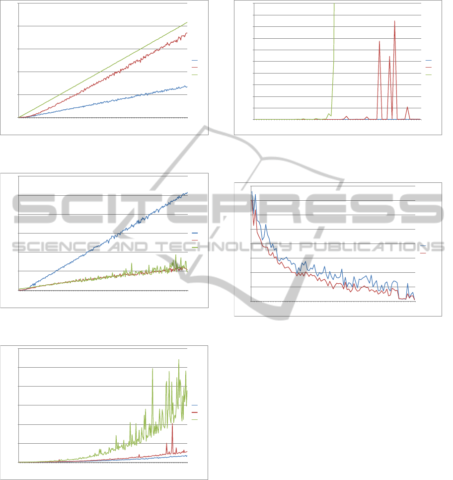
Briefly speaking, the experimental results con-
firmed the hypotheses. As depicted in figure 2, the
Right Shift Affected algorithm is far better when
optimizing the distance function f
2
, but the STN-
Recovery algorithm is significantly better when op-
timizing the distance function f
3
, as shown in figure
3. As far as function f
1
is concerned (which is the
total sum of shifts), the STN-Recovery algorithm out-
performs the Right Shift Affected, but the difference
is negligible.
The Right Shift Affected algorithm is somewhat
faster than STN-Recovery (see figure 4), however,
STN-Recovery has the following advantage. The al-
gorithm always allocates the leftmost connected com-
ponent that has not been allocated yet, therefore,
when the algorithm is allocating the connected com-
ponentwith the leftmostactivity that has the MinStart
value t, the schedule is not going to be modified be-
fore time point t. This allows the system to keep ex-
ecuting an ongoing schedule even if it has not been
ICAART2015-InternationalConferenceonAgentsandArtificialIntelligence
128

0
500
1000
1500
2000
2500
8
56
104 152 200 248 296 344 392 440
488
536 584 632 680 728 776 824 872 920 968
1016 1064 1112 1160 1208 1256 1304 1352 1400 1448 1496 1544 1592 1640 1688 1736 1784 1832 1880 1928 1976
2024
2072
number of moved activities
activities
RSA
STN
TR
Figure 2: The number of shifted activities for Right Shift
Affected, STN-Recovery, and Total Rescheduling.
0
200
400
600
800
1000
1200
8
56
104 152 200 248 296 344 392
440
488 536 584 632 680 728 776 824 872 920 968
1016 1064 1112 1160 1208 1256 1304 1352 1400 1448 1496 1544 1592 1640 1688 1736 1784 1832 1880 1928
1976
2024 2072
maximum time shift
activities
RSA
STN
TR
Figure 3: The biggest shift of an activity for Right Shift
Affected, STN-Recovery, and Total Rescheduling.
0
1000
2000
3000
4000
5000
6000
8
56
104 152 200 248 296 344 392
440
488 536 584 632 680 728 776 824 872 920 968
1016 1064 1112 1160 1208 1256 1304 1352 1400 1448 1496 1544 1592 1640 1688 1736 1784 1832 1880 1928
1976
2024 2072
runtime [ms]
activities
RSA
STN
TR
Figure 4: Run times for Right Shift Affected, STN-
Recovery, and Total Rescheduling.
completely recovered yet.
The dependencies on the density of constraints
showed no tendency. However, one might wonder
how the algorithms perform as the size of connected
components increases. As depicted in figure 5, there
are alarmingly longer run-times of STN-Recovery for
some models, but exponential growth is not apparent,
unlike in the case of total rescheduling, which turned
out to be useless by the component size of 33.
0
5000
10000
15000
20000
25000
30000
35000
40000
45000
50000
1 3 5 7 9 11 13 15 17 19 21 23 25 27 29 31 33 35 37 39 41 43 45 47 49 51 53 55 57 59 61 63 65
runtime [ms]
activities in one component
RSA
STN
TR
Figure 5: Run times for Right Shift Affected, STN-
Recovery, and Total Rescheduling, dependent on the num-
ber of activities in one component.
0
100
200
300
400
500
600
700
800
6 9 12 15 18 21 24 27 30 33 36 39 42 45 48 51 54 57 60
63
66 69 72 75 78 81 84 87 90 93 96 99
runtime [ms]
resources
CBJ
CBJBM
Figure 6: Run times for Conflict-Directed Backjumping and
Conflict-Directed Backjumping with Backmarking.
As far as the backmarking technique is concerned,
it brought some saving of time as expected, because
determining availability of a resource is carried out in
logarithmic time in the number of activities on the re-
source. On the other hand, as the number of resources
in the model decreases below a certain number, one
might expect backmarking to become counterproduc-
tive owing to the overhead costs. Nevertheless, ac-
cording to figure 6, backmarking pays regardless of
the number of resources in the model.
7 CONCLUSIONS
This paper proposed two different methods to han-
dle a resource failure, i.e., a disruption when a re-
source suddenly cannot be used anymore by any ac-
tivity, which may occur during a schedule execution.
The first method takes the activities that were to be
processed on a broken machine, reallocates them, and
then it keeps repairingviolated constraints until it gets
a feasible schedule. This approach is suitable when
ReactiveRecoveryfromMachineBreakdowninProductionSchedulingwithTemporalDistanceandResourceConstraints
129

it is desired to move as few activities as possible;
however, the question whether the algorithm always
ends is still open. The second method deallocates a
subset of activities and then it allocates them back
through Conflict-Directed Backjumping with Back-
marking. This approach is useful when the intention
is to shift activities by a short time distance, regard-
less of the number of moved activities.
The main shortcoming is that if there is no feasi-
ble recovery of the ongoing schedule, neither of the
methods is able to quickly and securely report it. In
real-life environments, however, the schedule recov-
erability from the breakdown of any particular ma-
chine is often known (for instance the minimum re-
quired number of available resources of each resource
group may be obvious) or can be computed before the
schedule execution begins.
Both suggested algorithms may be easily adapted
to handle the models with arbitrary resource groups,
and also to cope with another disturbance – hot order
arrival (Vlk, 2014).
Further investigation is needed for determining
the conditions under which a schedule is recoverable.
Next, it may be of interest to generalize the algorithms
for models that involve for example interruptibility of
activities, various speeds of resources, setup times of
resources or calendars of availabilities of resources.
ACKNOWLEDGEMENTS
Research is supported by the Czech Science Foun-
dation under the project P103/10/1287 and by the
Charles University in Prague, project GA UK No.
178915.
REFERENCES
Abumaizar, R. J. - Svestka, J. A. (1997). Rescheduling Job
Shops under Random Disruptions. International Jour-
nal of Production Research, 35(7), 2065-2082.
Bart´ak, R.- Jaˇska, M. - Nov´ak, L. - Rovensk´y, V. - Skalick´y,
T. - Cully, M. - Sheahan, C. - Thanh-Tung, D. (2012).
FlowOpt: Bridging the Gap Between Optimization
Technology and Manufacturing Planners. Proceed-
ings of ECAI 2012, pp. 1003-1004, IOS Press.
Brailsford, S.C. - Potts, Ch.N. - Smith, B. M. (1999). Con-
straint satisfaction problems: Algorithms and appli-
cations. European Journal of Operational Research
119, 557-581.
Dechter, R. - Meiri, I. - Pearl, J. (1991). Temporal constraint
networks. Artificial Intelligence 49(1-3), 61–95.
Kondrak, G. - Beek, P. van (1997). A Theoretical Evalu-
ation of Selected Backtracking Algorithms. Artificial
Intelligence 89, 365-387.
Ouelhadj, D. - Petrovic, S. (2009). A survey of dy-
namic scheduling in manufacturing systems. Journal
of Scheduling, v.12 n.4, p.417-431.
Planken, L. R. (2008). New Algorithms for the Simple Tem-
poral Problem. Delft, the Netherlands, 75 p. Master’s
thesis, Delft University of Technology.
Raheja, A. S. - Subramaniam, V. (2002). Reactive recovery
of job shop schedules – a review. International Jour-
nal of Advanced Manufacturing Technology, 19, 756-
763.
Skalick´y, T. (2011). Interactive Scheduling and Visualisa-
tion. Prague, 95 p. Master’s thesis, Charles University
in Prague.
Smith, S.F. (1994). Reactive Scheduling Systems. In: D.
Brown and W. Scherer (eds.), Intelligent Scheduling
Systems.
Vieira, G. - Herrmann, J. - Lin, E. (2003). Rescheduling
manufacturing systems: a framework of strategies,
policies, and methods. Journal of Scheduling 6: 39-
62, Kluwer Acad. Publishers.
Vlk, M. (2014). Dynamic Scheduling. Prague, 72 p. Mas-
ter’s thesis, Charles University in Prague.
ICAART2015-InternationalConferenceonAgentsandArtificialIntelligence
130