Automatic Image Annotation Using Convex Deep Learning Models

Niharjyoti Sarangi and C. Chandra Sekhar

Department of CSE, Indian Institute of Technology Madras, Chennai, India

Keywords:

Image Annotation, Tensor Deep Stacking Networks, Kernel Deep Convex Networks, Deep Convolutional

Network, Deep Learning.

Abstract:

Automatically assigning semantically relevant tags to an image is an important task in machine learning. Many

algorithms have been proposed to annotate images based on features such as color, texture, and shape. Success

of these algorithms is dependent on carefully handcrafted features. Deep learning models are widely used to

learn abstract, high level representations from raw data. Deep belief networks are the most commonly used

deep learning models formed by pre-training the individual Restricted Boltzmann Machines in a layer-wise

fashion and then stacking together and training them using error back-propagation. In the deep convolutional

networks, convolution operation is used to extract features from different sub-regions of the images to learn

better representations. To reduce the time taken for training, models that use convex optimization and kernel

trick have been proposed. In this paper we explore two such models, Tensor Deep Stacking Network and

Kernel Deep Convex Network, for the task of automatic image annotation. We use a deep convolutional

network to extract high level features from raw images, and then use them as inputs to the convex deep

learning models. Performance of the proposed approach is evaluated on benchmark image datasets.

1 INTRODUCTION

Developing techniques for efﬁcient extraction of us-

able and meaningful information has become increas-

ingly important with the explosive growth of digital

technologies. Low level features like color, texture

and shape can be used to classify images into differ-

ent categories. However, in many cases it is not suit-

able to use a single class label because of the pres-

ence of more than one semantic concept in an image.

One way to handle this is by assigning multiple rele-

vant keywords to a given image, reﬂecting its seman-

tic content. This is often referred to as image annota-

tion.

Learning techniques such as Binary Relevance

(Boutell et al., 2004) and Classiﬁer Chains (Read

et al., 2011), transform an annotation task into a

task of binary classiﬁcation. Another approach to

tackle the problem of annotation is by adapting pop-

ular learning techniques to deal with multiple labels

directly (Tsoumakas and Katakis, 2007; Zhang and

Zhou, 2014). Multi Label k-Nearest Neighbors (ML-

kNN) (Zhang and Zhou, 2007), Multi Label Decision

Tree (ML-DT) (Vens et al., 2008) and Rank-SVM

(Elisseeff and Weston, 2001) are some of the com-

monly used methods in this category. Rank-SVM is

a ranking based approach coupled with a set size pre-

dictor which uses Support Vector Machines to min-

imize the ranking loss while having a large margin.

Among other models, semantic space auto-annotation

model (Hare et al., 2008) constructs a special form of

a vector space, called a semantic space, from the la-

bels associated with the images. Images are projected

into this space in order to be retrieved or annotated.

Latent semantic analysis (Hofmann, 1999) is used to

build this space. The success of these techniques is

largely dependent on the effectiveness of the features

used.

Learning representations of the data that makes it

easier to extract useful information is highly desirable

(Bengio et al., 2013) for developing a good classiﬁca-

tion or annotation framework. Deep learning mod-

els are the commonly used techniques for learning

representation from raw data. These models aim at

learning feature hierarchies with features from higher

levels of the hierarchy formed by the composition of

lower level features, as illustrated in Figure 1.

Deep learning models such as Deep Belief Net-

works (DBN) (Hinton and Salakhutdinov, 2006) and

Deep Boltzmann Machines (DBM) (Salakhutdinov

and Hinton, 2009; Ranzato et al., 2010; Montavon

et al., 2012) have performed well in classiﬁcation and

Sarangi N. and Chandra Sekhar C..

Automatic Image Annotation Using Convex Deep Learning Models.

DOI: 10.5220/0005216700920099

In Proceedings of the International Conference on Pattern Recognition Applications and Methods (ICPRAM-2015), pages 92-99

ISBN: 978-989-758-077-2

 2015 SCITEPRESS (Science and Technology Publications, Lda.)

...

Input Layer

Hidden Layers

Output Layer (Optional)

These learn more abstract features.

This has raw sensory data or extracted features as input.

Figure 1: Scheme of learning representations in a multilay-

ered network. Raw pixel values or extracted features are

given as input. The input layer is followed by multiple hid-

den layers that learn increasingly abstract representation.

recognition tasks (Le Roux and Bengio, 2008). These

models are formed by pre-training individual layers

(Hinton et al., 2006a) and then stacking together and

training them using error back-propagation. Each

layer of a DBN consists of an energy-based model

known as Restricted Boltzmann Machine (RBM). An

RBM is trained using contrastive divergence to ob-

tain a good reconstruction of the input data (Hinton

et al., 2006b). Contrastive divergence and error back-

propagation are computationally complex methods.

In Deep Convolutional Networks (LeCun et al., 2010;

Lee et al., 2009; Krizhevsky et al., 2012), convolu-

tion operation is used to extract features from differ-

ent sub-regions of an image to learn a better repre-

sentation. Although Deep Convolutional Networks

are trained completely using error back-propagation,

they use sub-sampling layers to reduce the number

of inputs to each layer. To solve the issue of com-

plexity, a model known as Deep Stacking Network

(DSN) (Deng et al., 2012b) that consists of many

stacking modules was recently proposed. Each mod-

ule is a specialized neural network consisting of a

single non-linear hidden layer and linear input and

output layers. Since convex optimization is used to

speedup the learning in each module, this model is

also called as Deep Convex Network (DCN) (Deng

and Yu, 2011). Tensor Deep Stacking Networks (T-

DSN) (Hutchinson et al., 2013) , introduced as an ex-

tension of the DSN architecture, captures better rep-

resentations by using two sets of nonlinear nodes in

the hidden layer. The T-DSN model has been shown

to perform better than the DSN model for image clas-

siﬁcation and phone recognition tasks. Kernel Deep

Convex Network(K-DCN) (Deng et al., 2012a) on the

other hand uses kernel trick so that the number of hid-

den nodes in each module is unbounded.

In this paper, we propose a framework that uses

convex deep learning models (T-DSN and K-DCN)

for the task of image annotation. We also propose us-

ing the features extracted from a Deep Convolutional

Network as input to the convex models. The remain-

der of this paper is organized as follows: Section 2

gives a brief discussion on T-DSN and K-DCN. In

Section 3 we describe the details of our experiments

and compare the results with the existing methods.

2 CONVEX DEEP LEARNING

MODELS

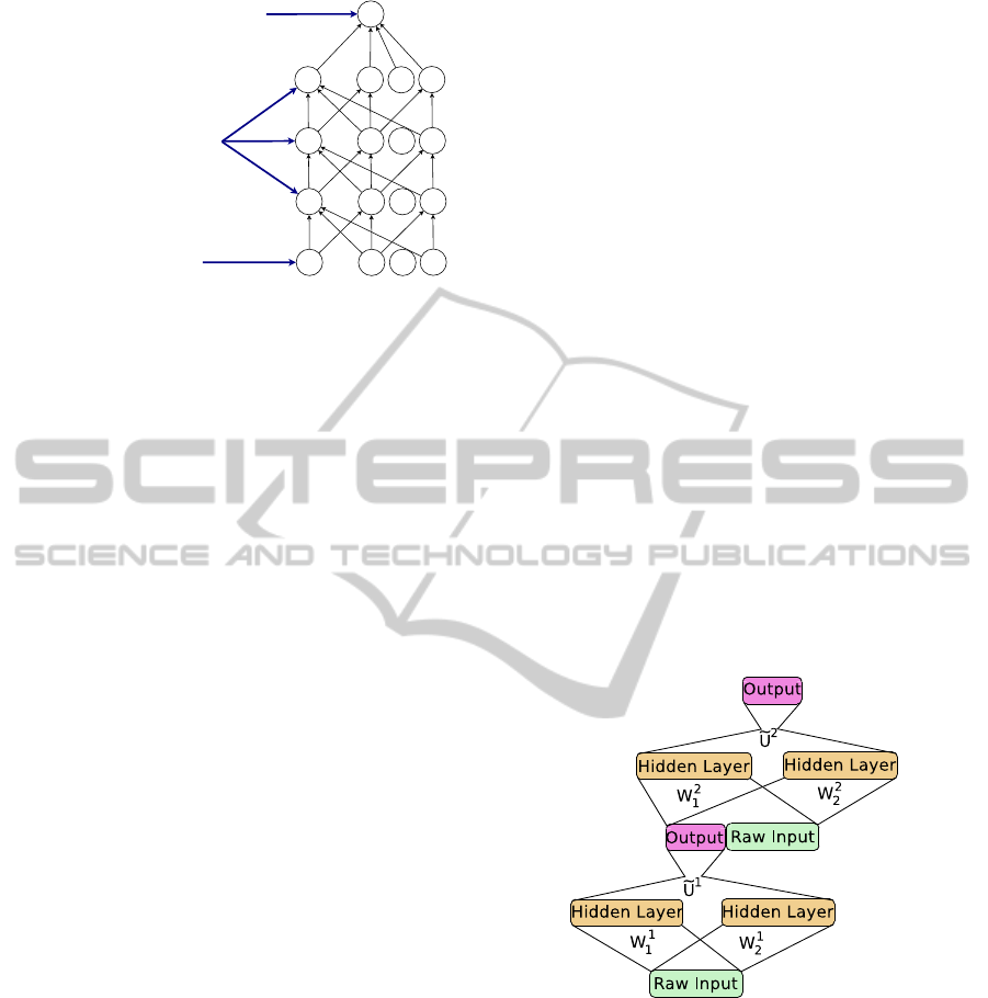
2.1 Tensor Deep Stacking Networks

A tensor deep stacking network is a generalized form

of a deep stacking network. The input data is provided

to the nodes in the input layer of the ﬁrst module. The

input to the higher modules is obtained by appending

output from the module just below it to the original

input data. Unlike DSN, each module of TDSN has

two sets of hidden layer nodes and thus, two sets of

connections between the input layer and the hidden

layer as shown in Figure 2. The output layer nodes

are bilinearly dependent on the hidden layer nodes.

Figure 2: Architecture of tensor deep stacking network.

Let the target vectors t be arranged to form the

columns of matrix T, the input data vectors v be ar-

ranged to form the columns of matrix V, and H

and

denote the set of matrices of the outputs of the

hidden units. There are two sets of lower weight pa-

rameters (W

and W

). They are associated with con-

nections from the input layer to the two hidden layers

containing L

and L

sigmoidal nodes respectively.

Since the hidden layers contain sigmoidal nodes,

the output of a hidden layer can be expressed as:

= logistic(W

(1)

AutomaticImageAnnotationUsingConvexDeepLearningModels

Let h

be the vector of outputs from the ﬁrst set of

hidden nodes and h

be the vector of outputs from the

second set of hidden nodes. Let h

be the i

entry in

and h

be the j

entry in h

If C is the number of nodes in the output layer,

weights of connections from hidden layers to the

output layer are represented as a tensor U ∈ R

× R

. The tensor U can be considered as a 3-

dimensional matrix.

Let y

denote the output of k

node in output

layer. The output vector can be obtained by comput-

ing (U ×

) ×

where ×

stands for multiplica-

tion along the i

dimension. In a simpliﬁed notation

∑

i=1

∑

j=1

ijk

(2)

Let

h = h

⊗ h

where ⊗ is the Kronecker product. Let

be the vec-

torized version of matrix U

in which all columns are

appended to form a single vector. The matrix U

obtained by setting the third dimension of tensor U

equal to k. Hence, length of

is L

. Now, we can

rewrite equation (2) as,

h (3)

Arranging all

’s for k = 1, 2, ...,C, into a matrix

= [

...

], the overall prediction becomes

y =

h (4)

where y is the estimate of target vector t.

Thus, bilinear mapping from two hidden layers

can be seen as a linear mapping from an implicit hid-

den representation

h. Aggregating the implicit hidden

layer representations for each of the N instances into

the columns of an L

× N matrix

H, we obtain

Y =

H (5)

where

H contains h

in k

column.

The convex formulation for

U in this case is,

min

H − Tk

(6)

where k.k

represents the squared norm operation.

Solving the optimization (6) we get:

= T

(

)

−1

(7)

We see that the output of each hidden node in ﬁrst

layer appears L

number of times in

h. So, we have

to add errors due to all those terms in order to get

the error caused by this particular node. Hence, the

equation for weight update needs to be modiﬁed to

account for this and the modiﬁed equations are:

∆W

= ηV[H

◦ (Γ− H

) ◦ Ψ

] (8)

∆W

= ηV[H

◦ (Γ− H

) ◦ Ψ

] (9)

Here ◦ is the element-wise multiplication of two ma-

trices, Γ is a matrix of all ones, η is the learning rate

and

∑

k=1

((i−1)L

+k),n

∑

k=1

((i−1)L

+k),n

(10)

Θ = 2

(

)(T

) − 2T

) (11)

Here H

is the matrix of outputs of nodes in the ﬁrst

hidden layer, H

is the matrix of outputs of nodes in

the second hidden layer. The dimensions of matrices

and Ψ

are N × L

and N × L

respectively. Each

of these two matrices Ψ

and Ψ

acts as a bridge be-

tween high dimensional implicit representation

h and

low dimensional representations u and v.

Since T-DSN uses convexoptimization techniques

to directly determine the upper-layer weights, the

training time is greatly reduced. However, computing

the lower-layer weights is still an iterative process.

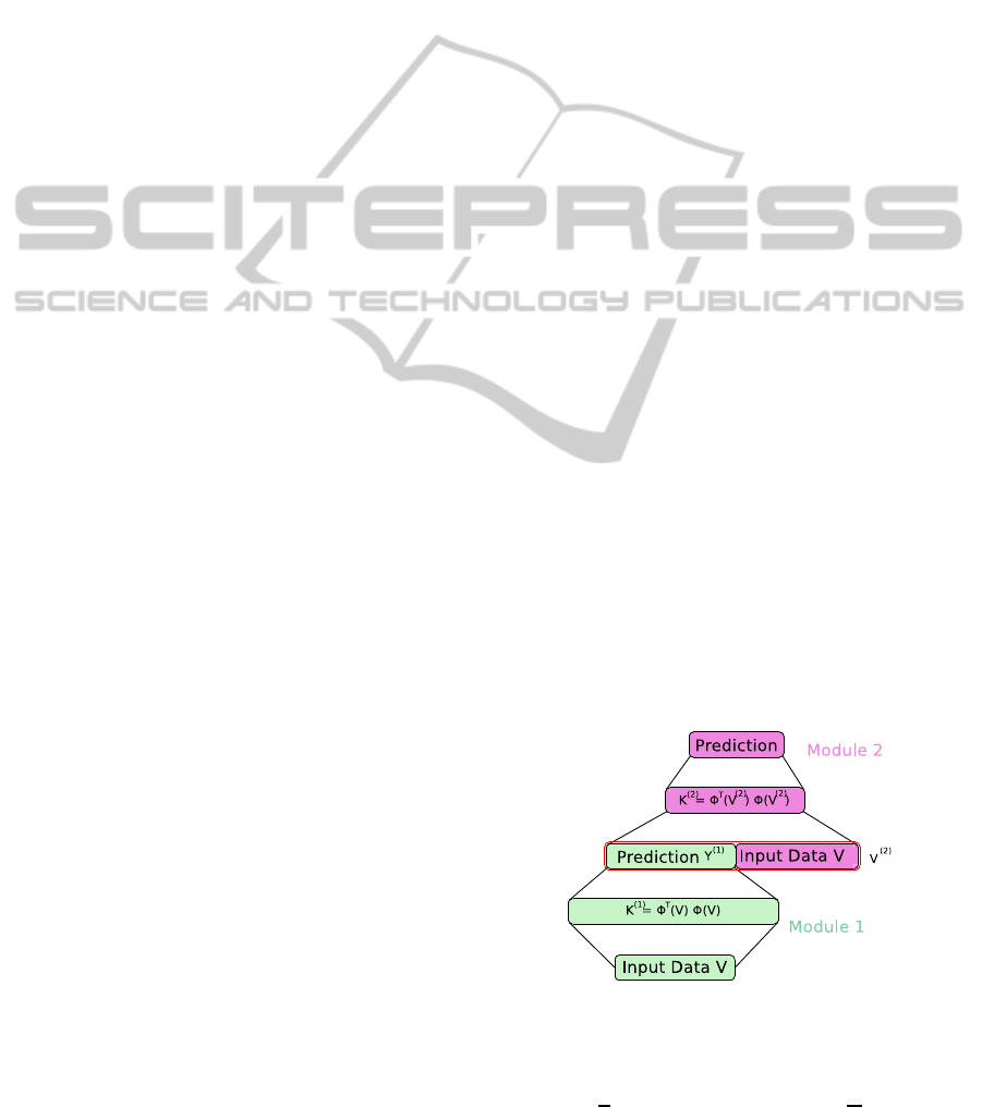
2.2 Kernel Deep Convex Networks

A kernel deep convex network (K-DCN), like a T-

DSN, is composed by stacking of shallow neural net-

work modules. This model completely eliminates the

non-convexlearning for the lower-layerweights using

the kernel trick. In case of K-DCN, a regularization

term C is included in the expression for computing the

upper-layer weights U. This modiﬁcation helps bound

the values of elements of U and prevents the model

from over-ﬁtting on the training data.

Figure 3: Architecture of kernel deep convex network with

two modules.

The formulation for U takes the form of,

min

[

∗ Tr{(Y − T)

(Y − T)} +

ICPRAM2015-InternationalConferenceonPatternRecognitionApplicationsandMethods

where Y is the predicted output for the output nodes

and T is the target output. The closed form expres-

sion for U is obtained by solving this minimization as

follows :

U = (CI + HH

)

−1

(12)

The output of the given module of KDCN is given

by,

= TH

(CI + HH

)

−1

(13)

The sigmoidal function of hidden units is replaced

with a generic nonlinear mapping function Φ(v) from

the raw input features v. The mapping Φ(v) will have

high-dimensionality (possibly inﬁnite) which is deter-

mined implicitly by a chosen kernel function. The

unconstrained optimization problem can be reformu-

lated as follows :

min

[

∗ Tr{(Y − T)

(Y − T)} +

subject to

T − U

G(V) = Y − T

where columns of G(V) are formed by applying the

transformation Φ(.) on each input v. Solving this

problem gives

U = G(V)(CI + K)

−1

(14)

where K = G

(V)G(V) is the kernel gram matrix of

Finally, for each new input vector v in the test set,

the prediction of KDCN module is given by

y(v) = U

Φ(v) = T(CI + K)

−1

(v) (15)

Here k(v) is the kernel vector such that k

(v) =

k(v

, v) and v

is a vector from training set.

For the subsequent modules, the output of nodes

in the output layer is appended with the raw input.

For l

module (l > 2) equation (14) is valid with a

slight modiﬁcation in the kernel function to account

for this extra input as follows :

K = G

(Z)G(Z) (16)

where Z = V|Y

(l−1)

(l−2)

|....|Y

, Y

is the predic-

tion of module m, and U|V represents the concatena-

tion of U and V.

Using the equations (15) and (16) we eliminate the

need of back-propagationand get a convexexpression

for training the model. The KDCN model combines

the power of deep learning and kernel learning in a

principled way. It is fast because there is no back-

propagation.

2.3 Framework for Image Annotation

If a concept is present in an image, the corresponding

bit in a binary target output vector t is turned on. Each

module of a T-DSN is trained to predict t. Once the

module is trained and the weights W

, W

, and U are

learned, equation (4) is used to compute the estimated

output. For the higher modules, the input data is con-

catenated with the output of the module below it (or

with the output of n modules below it) and used as an

augmented input. This process is repeated for all the

modules and the output obtained at the last module

is retained. Similarly, in case of a K-DCN, equation

(15) is used to ﬁnd predictions for each module.

One of the following methods to obtain the anno-

tation labels from the outputs of a model is used.

1. A threshold value is decided empirically using a

held-out validation set. In the estimated output

vectors, if the posterior probability value for a par-

ticular concept exceeds the threshold, it is consid-

ered as an annotation label for the image.

2. Based on the average number of labels present in

the images, a value k is selected. An image is an-

notated with those concepts that correspond to the

top k values in the estimated output vector.

3 EXPERIMENTS AND RESULTS

In this section, we present the details of image anno-

tation datasets used and the experimental results for

T-DSN and K-DCN. We compare the performance of

these models with the state-of-the-art performance.

3.1 Experimental Setup

We used MATLAB on an Intel i7 8-core CPU with 16

GB of RAM for running the Rank-SVM. For T-DSN

and K-DCN, we used NVIDIA Tesla K20C GPU with

CUDA.

In order to reduce the number of multiplications in

the computation of

Θ, equation (11) is re-written as:

Θ = 2(

− T

)(T

)

= 2(

− T

)

(17)

In order to reduce the memory requirements for

the computation of

Θ, equation (17) is parenthesized

as follows:

Θ = 2(

(

) − T

)

(18)

In this order of multiplication, we avoid comput-

ing

H, which is a N × N matrix. In general, the

AutomaticImageAnnotationUsingConvexDeepLearningModels

value of N is large (20,000 - 50,000). Accommodat-

ing such a large matrix in the GPU memory is prob-

lematic. Many matrices are reused in the process of

training. Matrices are allocated memory only when

required and freed immediately after their use in or-

der to make the best use of memory available.

For K-DCN, we used three different types of ker-

nel functions, namely, Gaussian kernel, Polynomial

kernel and Histogram Intersection Kernel (HIK). The

kernel parameters and regularization parameter were

tuned to obtain a range of values for the ﬁrst mod-

ule. For the later modules, the tuning is done with

respect to the range of parameters obtained for the

previous module, and a set of globally optimum pa-

rameters was obtained.

3.2 Feature Extraction

We used a deep convolutionalnetwork to obtain a use-

ful representation from an image. A deep convolu-

tional network consists of several layers. A convolu-

tional layer consists of a rectangular grid of neurons.

Each neuron takes inputs from a rectangular section

of the previous layer. The weights for this rectangular

section are constrained to be the same for each neuron

in the convolutional layer. Constraining the weights

makes it work like many different copies of the same

feature detector applied to different positions. This

constraint also helps in restricting the number of pa-

rameters. The output of a neuron in the convolutional

layer, l for a ﬁlter of size (m∗ n) is given by

= f(

∑

x=0

∑

y=0

(l−1)

(x+i)(y+ j)

) (19)

where f(x) = log(1 + e

). This nonlinearity was

approximated using a simpler function, f(x) =

max(0, x), which is known as the rectiﬁer function.

The nodes that use the rectiﬁer function are referred

to as Rectiﬁed Linear Units (ReLU). Use of ReLU re-

duced the time taken signiﬁcantly.

The pooling layer takes outputs of small rectangu-

lar blocks in the convolutional layer and subsamples it

to produce a single output from that block. The pool-

ing layer can take the average, or maximum, or learn

a linear combination of outputs of the neurons in the

block. In all our experiments, we used max-pooling.

Pooling helps the network achieve small amount of

translational invariance at each level. Also, it reduces

the number of inputs to the next layer. Finally, after

two convolutional and max-pooling layers, we added

two fully connected layers. The activity of the nodes

in the last fully connected layer was used as input to

the T-DSN and K-DCN models.

Apart from this, we also used the SIFT features

(Lowe, 2004) as input to the deep learning models.

3.3 Datasets Used

We test our models with two real-world datasets that

contain color images with their annotations: Uni-

versity of Washington annotation benchmark dataset

(Washington, 2004) and the MIRFLICKR-25000 col-

lection (Huiskes and Lew, 2008).

The Washington dataset had 1109 color images

corresponding to 22 different categories with an av-

erage annotation length of 6. Out of all the concepts

available, we selected only 45 concepts that had more

than 25 images associated with each of them. The list

of these 45 concepts is given in Table 1.

Table 1: List of 45 concepts selected for our study on Uni-

versity of Washington annotation benchmark dataset.

trees bushes grass sidewalk ground

rock ﬂowers camp sky trees

trunk people water dog woman

street cars pole house beach

ocean clouds mountain river building

lantern window bridge band man

stone Snow Boats sun Huskies

football Stadium stand ﬁeld hiker

mosque frozen players temple smoke

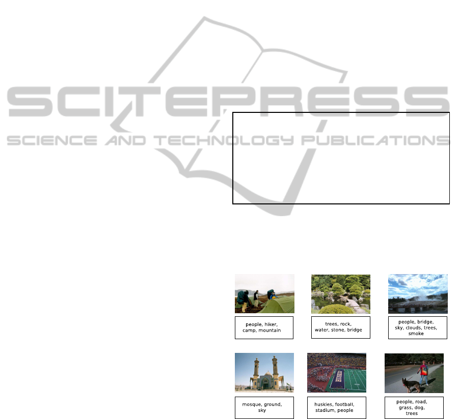
Some of the images from this dataset with their

annotation labels are shown in Figure 4. Because of

the small number of images, we do not use convolu-

tional features for this dataset.

Figure 4: Illustration of images with their annotation labels

from the University of Washington annotation benchmark

dataset.

MIRFLICKR-25000 is a database of 25,000 color

images belonging to various categories. The aver-

age number of tags per image is 9. Some of the im-

ages from this dataset with their annotation labels are

shown in Figure 5. For our studies, we consider the

ICPRAM2015-InternationalConferenceonPatternRecognitionApplicationsandMethods

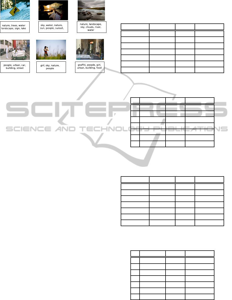
Figure 5: Illustration of images with their annotation labels

from the MIRFLICKR dataset.

30 most frequently occurring tags. These tags have at

least 150 images associated with each of them.

We randomly selected 30% of the images for test-

ing, and repeated our studies over 5 folds.

3.4 Results

A T-DSN consisting of 3 modules with 100 nodes in

each of the hidden layers was used on the University

of Washington dataset. In our experiments we ob-

served that having the same number of nodes in both

the sets of hidden nodes generally give a better per-

formance.

The precision, recall and F-measure for different

thresholds in the threshold based decision logic are

reported in Table 2.

We repeated the previous experiment with differ-

ent values of k in the top-k based decision logic, and

the precision, recall, and F-measure values are re-

ported in Table 3.

We repeated these experiments with K-DCN. Best

performance was observed for a Gaussian Kernel.

The results of these experiments are reported in Ta-

ble 4 and Table 5.

It is observed that the F-measure values for K-

DCN are slightly lower when compared with that for

T-DSN. One of the possible reasons for this could be

that the kernel parameters used might not be the best.

The state-of-the-art methods for image annotation,

namely, Rank-SVM and semantic space model give

F-measure values of 0.61 and 0.63 respectively. Fig-

ure 6 compares the actual annotation labels for some

randomly selected images in University of Washing-

ton dataset with the annotations generated by the T-

DSN model.

It is observed that the number of annotation labels

generated by the models were slightly higher than that

of the ground truth. In many cases, the extra labels are

somehow related to the image.

Table 2: Precision, recall, and F-measure for different

thresholds in the threshold based decision logic for anno-

tation of images in the University of Washington data with

T-DSN.

Threshold Precision Recall F-measure

0.20 0.50 0.87 0.64

0.25 0.58 0.81 0.67

0.30 0.63 0.75 0.68

0.35 0.68 0.70 0.68

0.40 0.72 0.64 0.67

0.45 0.73 0.58 0.64

0.50 0.75 0.47 0.58

Table 3: Precision, recall, and F-measure for different val-

ues of k in the top-k based decision logic for annotation of

images in the University of Washington data with T-DSN.

k Precision Recall F-measure

2 0.42 0.27 0.33

3 0.51 0.46 0.48

4 0.52 0.60 0.56

5 0.50 0.70 0.58

6 0.49 0.79 0.60

7 0.44 0.84 0.58

8 0.41 0.88 0.56

Table 4: Precision, recall, and F-measure for different

thresholds in the threshold based decision logic for anno-

tation of images in the University of Washington data with

K-DCN.

Threshold Precision Recall F-measure

0.20 0.39 0.90 0.54

0.25 0.50 0.84 0.63

0.30 0.52 0.81 0.63

0.35 0.59 0.76 0.66

0.40 0.64 0.68 0.66

0.45 0.73 0.59 0.65

0.50 0.77 0.49 0.59

Table 5: Precision, recall, and F-measure for different val-

ues of k in the top-k based decision logic for annotation of

images in the University of Washington data with K-DCN.

k Precision Recall F-measure

2 0.31 0.21 0.25

3 0.43 0.49 0.46

4 0.48 0.53 0.50

5 0.48 0.61 0.54

6 0.46 0.68 0.55

7 0.41 0.77 0.53

8 0.37 0.85 0.52

For the MIRFLICKR dataset, the study is carried

out using the SIFT features and convolutional fea-

AutomaticImageAnnotationUsingConvexDeepLearningModels

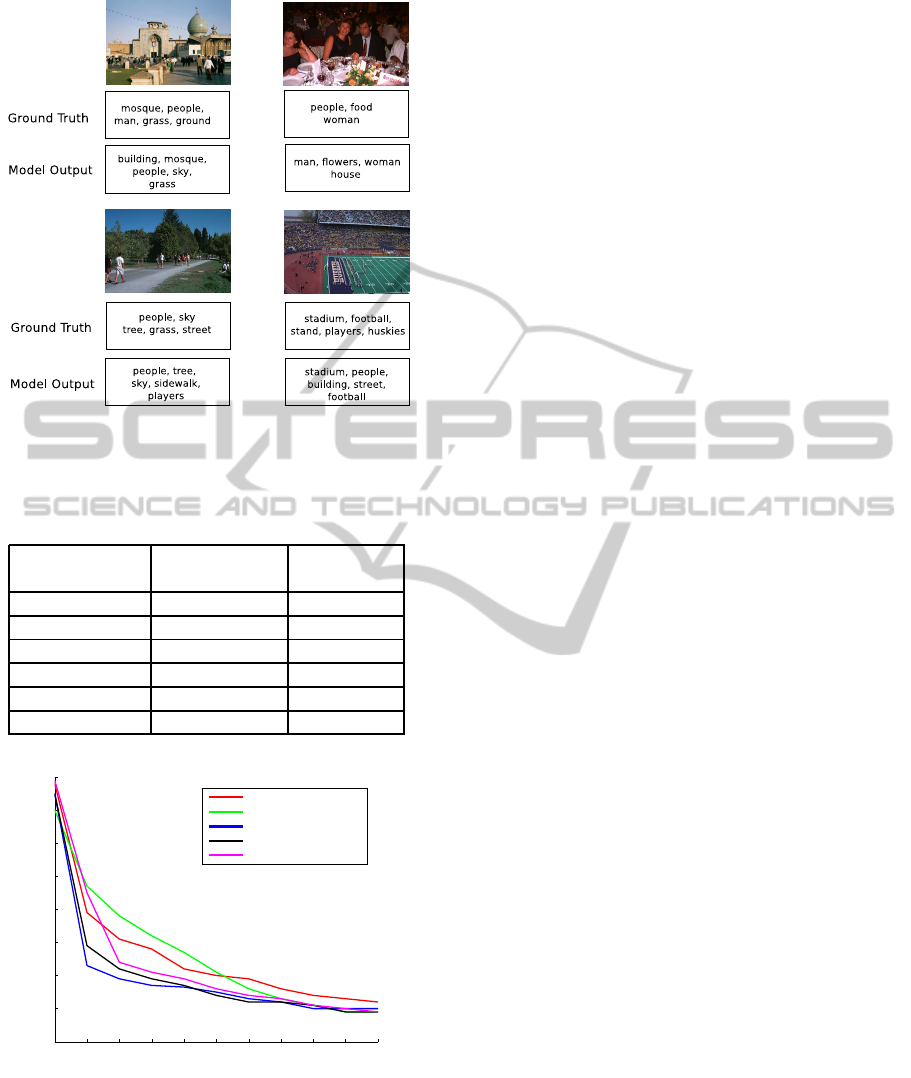
Figure 6: Illustration of images with actual annotation la-

bels and predicted annotation labels in the University of

Washington dataset with T-DSN.

Table 6: Performance comparison of models for image an-

notation task on MIRFLICKR dataset.

Model

Input

Features

F-Measure

Semantic Spae SIFT 0.26

Rank-SVM SIFT 0.25

TDSN SIFT 0.24

TDSN Convolutional 0.29

KDCN SIFT 0.26

KDCN Convolutional 0.34

0 0.1 0.2 0.3 0.4 0.5 0.6 0.7 0.8 0.9 1

0.1

0.2

0.3

0.4

0.5

0.6

0.7

0.8

Recall

Precision

Precision−Recall curves on MIRFLICKR dataset

T−DSN (Convolutional)

K−DCN (Convolutional)

K−DCN (SIFT)

T−DSN (SIFT)

Semantic Space (SIFT)

Figure 7: Precision-recall curves for different models on

MIRFLICKR dataset.

tures. Fig. 7 shows the precision-recall curves for dif-

ferent models. The best F-measure values for differ-

ent models are presented in Table 6.

It is observed that K-DCN and T-DSN perform

better with convolutional features. It is also noted that

convex deep learning methods perform better than the

semantic space annotation method.

4 SUMMARY AND

CONCLUSIONS

In this paper, we used the convex deep learning mod-

els, such as T-DSN and K-DCN for image annotation

tasks. We also used features extracted from a deep

convolutional network for this task. Through the ex-

perimental studies, it is observed that the T-DSN and

K-DCN models with convolutional features as input

give an improved performance. Once the convolu-

tional network is trained on a large set of images, it

is easy to extract features. The convex networks take

less time to train, making them useful for image an-

notation tasks in practice.

For the K-DCN model, we have used only a sin-

gle kernel function for a module. We can extend this

by using multiple types of kernel functions. Finding a

set of globally optimal parameters for K-DCN is dif-

ﬁcult. Similarly, for T-DSN we observed that having

different number of nodes in each hidden layer is not

beneﬁcial. However, we did not ﬁnd any criterion for

selecting the suitable number of hidden layer nodes.

A recipe for selecting the number of nodes in T-DSN

and globally optimum parameters for K-DCN will be

useful.

REFERENCES

Bengio, Y., Courville, A., and Vincent, P. (2013). Represen-

tation learning: A review and new perspectives. IEEE

Transactions on Pattern Analysis and Machine Intel-

ligence, 35(8):1798–1828.

Boutell, M. R., Luo, J., Shen, X., and Brown, C. M.

(2004). Learning multi-label scene classiﬁcation. Pat-

tern Recognition, 37(9):1757–1771.

Deng, L., T¨ur, G., He, X., and Hakkani-T¨ur, D. Z. (2012a).

Use of kernel deep convex networks and end-to-end

learning for spoken language understanding. In IEEE

Workshop on Spoken Language Technologies, pages

210–215.

Deng, L. and Yu, D. (2011). Deep convex network: A scal-

able architecture for speech pattern classiﬁcation. In

Interspeech.

Deng, L., Yu, D., and Platt, J. (2012b). Scalable stacking

and learning for building deep architectures. In Pro-

ceedings of the International Conference on Acous-

tics, Speech, and Signal Processing.

Elisseeff, A. and Weston, J. (2001). A kernel method for

multi-labelled classiﬁcation. In Advances in Neural

Information Processing Systems 14, pages 681–687.

ICPRAM2015-InternationalConferenceonPatternRecognitionApplicationsandMethods

Hare, J., Samangooei, S., Lewis, P., and Nixon, M. (2008).

Semantic spaces revisited: investigating the perfor-

mance of auto-annotation and semantic retrieval us-

ing semantic spaces. In Proceedings of the Interna-

tional conference on Content-based image and video

retrieval, pages 359–368.

Hinton, G. E., Osindero, S., and Teh, Y.-W. (2006a). A

fast learning algorithm for deep belief nets. Neural

Computation, 18(7):1527–1554.

Hinton, G. E., Osindero, S., Welling, M., and Teh, Y. W.

(2006b). Unsupervised discovery of nonlinear struc-

ture using contrastive backpropagation. Cognitive Sci-

ence, 30(4):725–731.

Hinton, G. E. and Salakhutdinov, R. R. (2006). Reducing

the dimensionality of data with neural networks. Sci-

ence, 313(5786):504–507.

Hofmann, T. (1999). Probabilistic latent semantic analysis.

In Proceedings of the Uncertainty in Artiﬁcial Intelli-

gence, pages 289–296.

Huiskes, M. J. and Lew, M. S. (2008). The mir ﬂickr re-

trieval evaluation. In Proceedings of the 2008 ACM

International Conference on Multimedia Information

Retrieval.

Hutchinson, B., Deng, L., and Yu, D. (2013). Tensor deep

stacking networks. IEEE Transactions on Pattern

Analysis and Machine Intelligence, 35(8):1944–1957.

Krizhevsky, A., Sutskever, I., and Hinton, G. E. (2012). Im-

agenet classiﬁcation with deep convolutional neural

networks. In Proceedings of the Neural Information

Processing System, volume 22, pages 1106–1114.

Le Roux, N. and Bengio, Y. (2008). Representational power

of restricted Boltzmann machines and deep belief net-

works. Neural Computation, 20(6):1631–1649.

LeCun, Y., Kavukcuoglu, K., and Farabet, C. (2010). Con-

volutional networks and applications in vision. In Pro-

ceedings of International Symposium on Circuits and

Systems, pages 253–256.

Lee, H., Grosse, R., Ranganath, R., and Ng, A. Y. (2009).

Convolutional deep belief networks for scalable unsu-

pervised learning of hierarchical representations. In

Proceedings of the 26th Annual International Confer-

ence on Machine Learning, pages 609–616.

Lowe, D. G. (2004). Distinctive image features from scale-

invariant keypoints. International Journal of Com-

puter Vision, 60(2):91–110.

Montavon, G., Braun, M. L., and Mller, K.-R. (2012). Deep

Boltzmann machines as feed-forward hierarchies. In

Proceedings of the International Conference on Ar-

tiﬁcial Intelligence and Statistics, volume 22, pages

798–804.

Ranzato, M., Krizhevsky, A., and Hinton, G. E. (2010). Fac-

tored 3-way restricted Boltzmann machines for mod-

eling natural images. Journal of Machine Learning

Research - Proceedings Track, 9:621–628.

Read, J., Pfahringer, B., Holmes, G., and Frank, E. (2011).

Classiﬁer chains for multi-label classiﬁcation. Ma-

chine Learning, 85(3):333–359.

Salakhutdinov, R. and Hinton, G. (2009). Deep Boltzmann

machines. In Proceedings of the International Con-

ference on Artiﬁcial Intelligence and Statistics, vol-

ume 5, pages 448–455.

Tsoumakas, G. and Katakis, I. (2007). Multi-label classi-

ﬁcation: An overview. International Journal of Data

Warehousing and Mining, 3(3):1–13.

Vens, C., Struyf, J., Schietgat, L., Dˇzeroski, S., and Block-

eel, H. (2008). Decision trees for hierarchical multi-

label classiﬁcation. Machine Learning, 73(2):185–

214.

Washington, U. (2004). Washington ground truth database.

http://www.cs.washington.edu/research/imagedatabase.

Zhang, M.-L. and Zhou, Z.-H. (2007). Ml-knn: A lazy

learning approach to multi-label learning. Pattern

Recognition, 40(7):2038 – 2048.

Zhang, M.-L. and Zhou, Z.-H. (2014). A review on multi-

label learning algorithms. IEEE Transactions on

Knowledge and Data Engineering, 26(8):1819–1837.

AutomaticImageAnnotationUsingConvexDeepLearningModels