A Comparative Study of Network-based Approaches for Routing in

Healthcare Wireless Body Area Networks

Pablo Adasme

, Rafael Andrade

, Janny Leung

and Abdel Lisser

Departamento de Ingenier´ıa El´ectrica, Universidad de Santiago de Chile, Avenida Ecuador 3519, Santiago, Chile

Departamento de Estat´ıstica e Matem´atica Aplicada, Universidade Federal do Cear´a,

Campus do Pici - Bloco 910, 60455-760, Fortaleza, Cear´a, Brazil

Department of Systems Engineering & Engineering Management, Chinese University of Hong Kong, Shatin, Hong Kong

Laboratoire de Recherche en Informatique, Universit´e Paris-Sud XI, Bˆatiment 650, 91405 Orsay Cedex, France

Keywords:

Healthcare Wireless Body Area Networks, Network Design Topology Approach, Mixed Integer Linear

Programming, Variable Neighborhood Search.

Abstract:

In this paper, we propose a minmax robust formulation for routing in healthcare wireless body area networks

(WBAN). The proposed model minimizes the highest power consumption of each bio-sensor node placed in

the body of a patient subject to ﬂow rate and network topology constraints. We consider three topologies in

the problem: a spanning tree, a star, and a ring topology as well. In particular, we use an equivalent poly-

nomial formulation of the spanning tree polytope (Yannakakis, 1991) to avoid having an exponential number

of cycle elimination constraints in the model. For the ring topology approach, we use constraints from the

well known mixed integer linear programming (MILP) formulation of the traveling salesman problem (Pataki,

2003). Thus, we compute optimal solutions and lower bounds directly using the MILP and linear program-

ming (LP) relaxations. Finally, we propose a Kruskal-based (Cormen et al., 2001) variable neighborhood

search metaheuristic to improve the solutions obtained with the star topology approach. Our preliminary nu-

merical results indicate that the tree approach is more convenient as it allows saving signiﬁcantly more power

while the ring approach is the most expensive one. They also indicate that the difference between the opti-

mal objective function values for the tree and star formulations is not very large and that VNS can improve

signiﬁcantly the solutions obtained with the star conﬁguration, although, at a higher computational cost.

1 INTRODUCTION

Wireless sensor networks (WSN) have been consid-

ered by the research community as one of the most

promising technologies within last decades. Mostly

due to the innumerable applications that can be re-

alized in order to enhance people’s quality of life.

Regarding healthcare systems, a major concern is

to deal with the problem of preventive monitoring

systems. Particularly, for elderly population whose

growth has signiﬁcantly increased around the globe

in last decades (Kinsella and Phillips, 2005). This

technology would also provide high quality care ser-

vices for young children in situations where both par-

ents are absent or in cases where people living in

rural areas can not reach hospitals and medical cen-

ters easily. Wireless body area networks (WBANs)

are composed of tiny biological sensors (bio-sensors)

which are placed in the body or in the clothes of a

person in order to remotely monitor healthcare status

conditions such as fever, blood pressure, body tem-

perature, heart rate, and so on. In a WBAN, pre-

serving the energy of the nodes is of great impor-

tance as their energy resources are limited. Addi-

tionally, an extremely low transmit power per node

is required in order to minimize interference. A com-

mon approach to deal with these problems is by im-

proving the performance of routing protocols. The

authors in (Fang and Dutkiewicz, 2009) propose an

efﬁcient medium access control (MAC) protocol re-

ferred to as BodyMAC. This protocol uses ﬂexible

bandwidth allocation to improve node energy efﬁ-

ciency. In (Kwak et al., 2009) the authors compare

and analyze different protocols from WBAN require-

ments whereas in (Huang et al., 2010) the authorspro-

pose a weighted random value protocol for multiuser

WBANs (WRAP). Finally, in (Elias and Mehaoua,

2012) the authors consider explicit mathematical pro-

125

Adasme P., Andrade R., Leung J. and Lisser A..

A Comparative Study of Network-based Approaches for Routing in Healthcare Wireless Body Area Networks.

DOI: 10.5220/0005218001250132

In Proceedings of the International Conference on Operations Research and Enterprise Systems (ICORES-2015), pages 125-132

ISBN: 978-989-758-075-8

 2015 SCITEPRESS (Science and Technology Publications, Lda.)

gramming formulations in order to efﬁciently design

optimal routing protocols in WBANs. WBAN is an

emerging research ﬁeld where new routing protocols

are mandatorily required to efﬁciently manage power

consumption in order to maximizing the lifetime of

the network. Additionally, ﬁnding the “best” net-

work topology conﬁguration in a WBAN is a very

important issue as it signiﬁcantly affects the proto-

col design as well as the overall performance of the

system. Finally, we mention that research on rout-

ing protocols for WBANs is still at its infancy. In

this paper, we present a minmax robust formulation

to optimally route sensed information by nodes in a

WBAN. The model minimizes the worst power con-

sumption of each bio-sensor subject to ﬂow rate and

network design topology constraints. We consider

three topologies in the problem: a spanning tree one,

a star one and a ring topology as well. In partic-

ular, we use an equivalent polynomial formulation

of the spanning tree polytope due to (Yannakakis,

1991) in order to avoid an exponential number of cy-

cle elimination constraints in the model. For the ring

topology approach, we use constraints from the well

known mixed integer linear programming(MILP) for-

mulation of the traveling salesman problem (Pataki,

2003). All the proposed models are formulated as

MILP models and thus we compute optimal solutions

and lower bounds directly using the MILP and lin-

ear programming (LP) relaxations, respectively. Fi-

nally, we propose a Kruskal-based variable neighbor-

hood search (VNS for short) metaheuristic to improve

the optimal solutions found with the star network con-

ﬁguration. We only consider a VNS procedure that

works with the tree topology approach as it is the one

that achieves signiﬁcantly more power savings. The

paper is organized as follows. Section 2 presents the

minmax robust formulation with the generic topology

constraint. In section 3, we present three MILP for-

mulations for each different topology. Subsequently,

in section 4 we present the Kruskal-based variable

neighborhood search procedure. Then, in section 5

we present preliminary numerical results in order to

compare the three MILP formulations together with

their LP relaxations. Next, we compare the VNS pro-

cedure with the star and tree MILP models. Finally,

section 6 concludes the paper.

2 PROBLEM FORMULATION

We model a ﬁxed WBAN by the means of a graph

G = (V = V

∪V

, E), where V

denotes a set of bio-

sensor nodes that sense and collect the data to be

transmitted while V

represents a sink node where all

the data is ﬁnally received. The set E represents the

set of edges in the graph G. For sake of simplicity, in

the remainder of the paper we assume that the graph

G is a complete graph. We consider the following

generic model we denote hereafter by P

min

{x,y}

max

{i∈V

}

∑

j∈V:(i, j)∈E

(1)

s.t.y

≤ Lx

, ∀i ∈ V

, j ∈ V : (i, j) ∈ E (2)

∑

j∈V:(i, j)∈E

−

∑

j∈V:( j,i)∈E

≥ r

∀i ∈ V

(3)

min

≤ r

≤ R

max

, ∀i ∈ V

(4)

Topology constraints on x

variables (5)

∈ {0, 1}, y

≥ 0, ∀i, j ∈ V (6)

In P

, variable x

= 1 if node i is connected to node

j and x

= 0 otherwise. Variable y

, i, j ∈ V repre-

sents the amount of ﬂow to be transmitted in edge

(i, j) ∈ E. The input parameter p

denotes the unitary

power required by node i to transmit a unit of ﬂow

. Hence, the objective function in (1) minimizes

the worst power consumption of each bio-sensor node

j ∈ V

overall edges (i, j) ∈ E. Constraint (2) implies

that y

should be equal to 0 if nodes i and j are not

connected, i.e. when x

= 0. Here, we assume that

each edge (i, j) ∈ E has a maximum link capacity de-

noted by L. Constraint (3) are ﬂow constraints forcing

each node i ∈ V

to transmit the sensed and collected

data through the network. For this purpose, we intro-

duce data rate variables r

for each node i ∈ V

. In

constraint (4), we further impose the condition that

each variable r

must be bounded as 0 ≤ R

min

≤ r

≤

max

, i ∈ V

where R

min

and R

max

are minimum and

maximum data rate parameters. In general, constraint

(4) is justiﬁed by the fact that low power medium ac-

cess control (MAC) and routing protocols allow vary-

ing the amount of data to be transmitted by a partic-

ular node depending on the quality of the channels

(Reusens et al., 2009; Ullah et al., 2012). Finally, con-

straint (5) represents a generic topology constraint we

should impose with variables x

as stated in section

In general, there exists several WBAN conﬁgura-

tions such as star, tree, or mesh type networks (Ullah

et al., 2012). The most common topology approach

is a star one where the nodes are connected to the

sink node in star manner (Ullah et al., 2012). How-

ever, the star conﬁguration follows a single hop strat-

egy which is not always the best choice. In (Reusens

et al., 2009), the authorsdiscuss about energy efﬁcient

topology designs for WBANs. They consider a tree

network topology and discuss on the energy savings

when using single hop and multi hop strategies. They

ICORES2015-InternationalConferenceonOperationsResearchandEnterpriseSystems

126

conclude that both single hop or multi hop strategies

can achieve energy savings under different conditions

(Reusens et al., 2009). In this paper, we compare

three topology approaches for WBANs, a tree one, a

star one and a ring topology as well. For this purpose,

we assume that all bio-sensors can communicate with

each other, i.e. we assume that the WBAN can be rep-

resented by means of a complete graph. Notice that

the parameter L in P

might lead to infeasible solu-

tions when using a multi hop strategy in some cases.

This can happen since the ﬂow constraints (3) accu-

mulate the amount of data to be transmitted from one

node to another. Whereas in the single hop strategy

this can rarely happen because the maximum capac-

ity of L is always larger than R

max

3 MILP FORMULATIONS

In this section, we present MILP formulations for the

spanning tree, star and ring network conﬁgurations.

For this purpose, we replace constraint (5) in model P

by different set of constraints depending on the topol-

ogy approach under consideration.

3.1 Spanning Tree Topology Approach

We propose the following spanning tree MILP formu-

lation and denote this model hereafter by P

as follows

min

{x,y,r,λ,t}

t (7)

s.t.

∑

j∈V:(i, j)∈E

≤ t, ∀i ∈ V

(8)

≤ Lx

, ∀i ∈ V

, j ∈ V : (i, j) ∈ E (9)

∑

j∈V:(i, j)∈E

−

∑

j∈V:( j,i)∈E

≥ r

∀i ∈ V

(10)

min

≤ r

≤ R

max

, ∀i ∈ V

(11)

kij

+ λ

kji

≥ x

, ∀k, i, j ∈ V (12)

∑

j∈V−{i}

kij

≤ 1, ∀k, i ∈ V, (k 6= i) (13)

kki

= 0, ∀k, i ∈ V, (k 6= i) (14)

∑

i, j∈V,i< j

= |V| − 1 (15)

∈ {0, 1}, y

≥ 0, ∀i, j ∈ V (16)

kij

∈ {0, 1}, ∀k, i, j ∈ V (17)

In particular, we replace the topology constraint (5)

in P

by the set of constraints (12)-(15) and (17) in

. This set of constraints characterizes the set of

all spanning trees in graph G (Yannakakis, 1991).

In P

, λ

kij

, ∀k, i, j ∈ V are binary decision variables

required to characterize the spanning tree polytope

(Yannakakis, 1991).

3.2 Star Topology Approach

Similarly, a star MILP formulation can be obtained

by replacing the topology constraint (5) by the set of

constraints (23)-(24) and (26). Thus, we state the fol-

lowing model we denote by P

as follows

min

{x,y,r,ϕ,t}

t (18)

s.t.

∑

j∈V:(i, j)∈E

≤ t, ∀i ∈ V

(19)

≤ Lx

∀i ∈ V

, j ∈ V : (i, j) ∈ E (20)

∑

j∈V:(i, j)∈E

−

∑

j∈V:( j,i)∈E

≥ r

∀i ∈ V

(21)

min

≤ r

≤ R

max

, ∀i ∈ V

(22)

≤ ϕ

, ∀i, j ∈ V, (i 6= j) (23)

∑

j∈V

= P (24)

∈ {0, 1}, y

≥ 0, ∀i, j ∈ V (25)

∈ {0, 1}, ∀ j ∈ V (26)

In P

, ϕ

, ∀ j ∈ V are binary decision variables re-

quired to characterize the feasible set of the star con-

ﬁguration. In particular, we require that the input pa-

rameter P = 1 in order to obtain a star network con-

ﬁguration centred at the sink node with all the edges

ﬂowing into it. Notice that the constraints (23)-(24)

can be merged into a single constraint as x

≤ 1, ∀i ∈

, j ∈ V

. However, we write them as such in or-

der to further consider the more general case when

1 < P ≤ |V| where |V| denotes the cardinality of V.

This means we relax the star topology condition and

allow a fully connected scenario, although at the cost

of ﬂooding the network.

3.3 Ring Topology Approach

Finally, we obtain a ring topology MILP formulation

by replacing the topology constraint (5) by the set of

constraints (32)-(36) and (38). In particular, we use

the set of constraints from the MILP formulation of

the traveling salesman problem (Pataki, 2003). Thus,

we formulate P

as follows

min

{x,y,r,u,t}

t (27)

s.t.

∑

j∈V:(i, j)∈E

≤ t, ∀i ∈ V

(28)

AComparativeStudyofNetwork-basedApproachesforRoutinginHealthcareWirelessBodyAreaNetworks

127

≤ Lx

∀i ∈ V

, j ∈ V : (i, j) ∈ E (29)

∑

j∈V:(i, j)∈E

−

∑

j∈V:( j,i)∈E

≥ r

∀i ∈ V

(30)

min

≤ r

≤ R

max

, ∀i ∈ V

(31)

∑

j∈V:(i, j)∈E

= 1, ∀i ∈ V (32)

∑

j∈V:(i, j)∈E

= 1, ∀i ∈ V (33)

= 1 (34)

2 ≤ u

≤ |V|, ∀i ∈ V, (i 6= 1) (35)

− u

+ 1 ≤ (|V| − 1)(1− x

∀i, j ∈ V, (i 6= 1), ( j 6= 1) (36)

∈ {0, 1}, y

≥ 0, ∀i, j ∈ V (37)

∈ Z

, ∀ j ∈ V (38)

In P

, u

, ∀i ∈ V are integer decision variables required

to characterize the feasible set of the traveling sales-

man problem (Pataki, 2003). Hereafter, we denote by

, LP

and LP

the LP relaxations of P

, P

and

, respectively. In the next section, we present a

Kruskal-based VNS algorithm that allows improving

the optimal solutions found with the star topology ap-

proach.

4 KRUSKAL-BASED VNS

ALGORITHM

Metaheuristics are simple algorithmic procedures

commonly used to ﬁnd near optimal (or suboptimal)

solutions for combinatorial optimization problems.

From a practical point of view, they have proven to

be highly effective when solving many of these hard

problems (Glover and Kochenberger, 2003). Espe-

cially when the dimensions of the problem increase

rapidly which is often the case in real world applica-

tions and where no solver is available to solve these

problems to optimality. The most frequently utilized

metaheuristics approaches are: genetic algorithms,

tabu search, ant colony system, particle swarm op-

timization, variable neighborhood search, simulated

annealing, among others. For a detailed explanation

on how these metaheuristics procedures work, we re-

fer the reader to the book in (Glover and Kochen-

berger, 2003). Basically, any metaheuristic approach

would serve to compute feasible solutions for our tree

MILP formulation. However, we choose VNS mainly

due to its simplicity and low memory requirements.

In particular, we adopt a reduced VNS strategy which

drops the local search phase of the basic VNS algo-

rithm as it is the most time consuming step (Hansen

and Mladenovic, 2001). In order to compute feasible

solutions for P

using a VNS approach, we observe

that for any ﬁxed assignment of variable x = ¯x in P

the problem reduces to solve the following linear pro-

gramming problem

min

{y,r,t}

t (39)

s.t.

∑

j∈V:(i, j)∈E

≤ t, ∀i ∈ V

(40)

≤ L¯x

, ∀i ∈ V

, j ∈ V : (i, j) ∈ E (41)

∑

j∈V:(i, j)∈E

−

∑

j∈V:( j,i)∈E

≥ r

∀i ∈ V

(42)

min

≤ r

≤ R

max

, ∀i ∈ V

(43)

≥ 0, ∀i, j ∈ V (44)

Hereafter, we denote by P

the LP problem (39)-

(44). Notice that the number of feasible assignments

for x in P

grows rapidly with the size of the instances.

Also notice that not all of these trees are feasible for P

since the capacity of each edge (i, j) ∈ E is limited by

L. We propose a Kruskal VNS approach to compute

feasible solutions for P

by randomly generating these

trees. VNS is a recently proposed metaheuristic ap-

proach (Hansen and Mladenovic, 2001) that uses the

idea of neighborhood change during the descent to-

ward local optima and to avoid the valleys that contain

them. The VNS approach we propose is presented in

Figure 1.

It receives an instance of problem P

as input and

provides a feasible solution for it. We denote by

( ˜x, ˜y, ˜r,

t) the ﬁnal solution obtained with the algo-

rithm where

t represents the objective function value

of P

. The algorithm is simple and works as fol-

lows. In Step 0, we initialize all the required vari-

ables. Then, in Step 1 we obtain an initial feasible

solution for the problem. For this purpose, we solve

and obtain the star network conﬁguration x = ¯x.

Then, we construct a cost vector c(i, j) for each edge

(i, j) ∈ E in such a way that x = ¯x can also be obtained

with Kruskal algorithm (Cormen et al., 2001). Find-

ing vector c(i, j) is required since we start our VNS

from the optimal solution of P

. Next, we save the

optimal objective function value of P

and the con-

structed vector c(i, j) as the bests found so far. We

deﬁne the neighborhood structure Ng(c) as the set of

neighbor vectors c

′

at a distance “h” from c where the

distance “h” corresponds to the number of entries in

vector c that are randomly swapped. There are |E|!

number of vectors c

′

in Ng(c) including c. Here, we

denote by |E| the cardinality of E. During the execu-

tion of the while loop in Step 2, the algorithm per-

ICORES2015-InternationalConferenceonOperationsResearchandEnterpriseSystems

128

Input: A problem instance of P

Output: A feasible solution ( ˜x, ˜y, ˜r,

t) for P

Step 0:

Time ← 0; H ← θ; min ← ∞

count ← 0; x

i, j

← 0, ∀i, j ∈ V

Step 1:

Solve P

; Let ( ¯x, ¯y, ¯r,

t) be the optimal solution of P

Construct a cost vector c = c(i, j), ∀(i, j) ∈ E

such that ¯x can be obtained with Kruskal algorithm.

min ←

t; cOpt(i, j) ← c(i, j), ∀(i, j) ∈ E

Step 2:

while (Time ≤ maxTime)

For h = 1 to H

choose randomly two different edges (i, j), (k, l) ∈ E

aux ← c(i, j); c(i, j) ← c(k, l); c(k, l) ← aux

end for

¯x ← Kruskal(G, c);

Solve the linear problem P

if(P

is feasible)

Let ( ¯y, ¯r,

t) be the optimal solution of P

with

objective function value

if(min >

min ←

t; cOpt(i, j) ← c(i, j), ∀(i, j) ∈ E

H ← 1; count ← 0

else

c(i, j) ← cOpt(i, j), ∀(i, j) ∈ E

count ← count +1

if (count > η)

if (H ≤ θ)

H ← H + 1

else

H ← 1

end if

count ← 0

end if

end while

Figure 1: VNS Algorithm.

forms a variable neighborhood search by randomly

swapping H ≤ θ valuesin vector c where θ represents

a parameter for the maximum number of swapping

movements. For each generated vector c

′

in Ng(c),

we ﬁnd a maximum spanning tree x = ¯x for G using

Kruskal algorithm. Then, for each found tree we solve

. If P

is feasible we obtain a new solution ( ¯y, ¯r,

with objective function value

t that we compare with

the best found so far. If this new solution is better, we

save

t and the new vector c(i, j), (i, j) ∈ E. In case P

is infeasible, the solution is discarded and not consid-

ered as a valid solution. Initially, H ← 1 while it is

increased in one unit when there is no improvement

after new “η” solutions have been evaluated. On the

other hand, if a new current solution is better than the

best found so far, then H ← 1, the new solution is

recorded and the process goes on. Note that if “η” so-

lutions have been evaluated without improvement and

if H = θ, then we also set H ← 1. This gives the pos-

sibility of searching in a loop manner from small to

large zones of the feasible space. The whole process

is repeated while the cpu time variable “Time” is less

than or equal to the maximum available “maxTime”.

5 NUMERICAL RESULTS

In this section, we present preliminary numerical re-

sults in order to compare the three MILP and LP for-

mulations. Then, we compare the proposed VNS al-

gorithm with the tree and star MILP formulations. Fi-

nally, we present numerical results for P

when in-

crementing the parameter P from 1 to |V|. The latter

resembles the case where a ﬂooding data transmission

situation is possible.

In our numerical tests, we assume that we only

have one node acting as a sink node which receives

all sensed and collected data sent by the remaining

nodes in the network. The input data is randomly gen-

erated as follows. The entries in matrix P

are drawn

from the interval (0, 2] (Elias and Mehaoua, 2012).

The maximum capacity for each edge (i, j) ∈ E is

set to L = 5Mbps and L = 10Mbps. The minimum

acceptable data rate generated by each node i ∈ V

is R

min

= 128 kbps whereas the maximum data rate

is set to R

max

= 512 kbps. The parameters θ and η

in the VNS algorithm were calibrated to the values

of θ =

|V|

and η = 50, respectively. A Matlab pro-

gram is implemented using CPLEX 12 to solve the

MILP and LP models. The numerical experiments

have been carried out on a Intel(R) 64bits core(TM)

with 3.4 Ghz and 8 GoBytes of RAM. In Table 1, col-

umn 1 shows the number of nodes considered for each

instance. Then, columns 2-5, 6-9, and 10-13 present

the optimal solutions, lower bounds, and cpu time in

seconds for the MILP and LP models respectively. Fi-

nally, in columns 14-16 we present gaps we compute



−LP



∗100 for P

, i= 1, 2, 3, respectively. With-

out loss of generality, we set the maximum available

cpu time for CPLEX to solve the MILP formulations

to 1 hour. From Table 1, we observe that the objec-

tive function values of the LP models are equal for all

the instances. On the opposite, the objective function

values of P

are lower than those obtained with P

and

for the instances 1-28 when using L = 5Mbps and

for the instances 1-22 when using L = 10Mbps, re-

spectively. For the instances 28-60, these values are

larger than P

and P

in most of the cases. This can

be explained by the fact that P

has more variables

and constraints than P

and P

. Consequently, it is

harder to ﬁnd feasible solutions with CPLEX in one

hour of cpu time. This is also conﬁrmed by the cpu

times required by CPLEX to solve LP

which is not

the case for LP

and LP

. In general, we observe that

the star topology approach is more restrictive than the

ring one. Similarly, the ring approach is more restric-

tive than the tree one. Indeed, the star topology ap-

proach represented by P

is not a combinatorial op-

timization problem when P = 1 as it has only one

AComparativeStudyofNetwork-basedApproachesforRoutinginHealthcareWirelessBodyAreaNetworks

129

Table 1: Numerical results for the MILP and LP formulations.

Randomly generated instances using L = 5Mbps.

|V| P

cpu P

cpu LP

cpu P

cpu LP

cpu P

cpu LP

Gap

(%) Gap

(%)

4 172.9123 128.3024 0.10 0.08 230.4138 128.3024 0.08 0.08 259.3685 128.3024 0.09 0.08 25.80 44.32 50.53

6 116.5641 98.4527 0.13 0.08 216.1431 98.4527 0.09 0.12 318.5687 98.4527 0.12 0.08 15.54 54.45 69.10

8 130.0117 98.1275 0.63 0.09 233.8014 98.1275 0.08 0.08 227.0687 98.1275 0.13 0.08 24.52 58.03 56.79

10 110.5027 78.2920 13.93 0.11 251.9203 78.2920 0.08 0.08 364.8153 78.2920 0.65 0.08 29.15 68.92 78.54

12 130.4526 97.9122 40.04 0.16 245.1696 97.9122 0.09 0.08 604.7503 97.9122 2.03 0.09 24.94 60.06 83.81

14 92.1095 71.1643 105.58 0.28 211.3495 71.1643 0.09 0.08 360.7896 71.1643 64.14 0.09 22.74 66.33 80.28

16 82.5006 59.6906 199.44 0.36 241.4101 59.6906 0.09 0.09 371.4371 59.6906 48.42 0.09 27.65 75.27 83.93

18 140.0872 86.8162 3600 0.45 245.6945 86.8162 0.08 0.08 522.0311 86.8162 142.72 0.11 38.03 64.66 83.37

20 141.7066 95.2401 3600 1.04 255.1937 95.2401 0.09 0.08 628.2930 95.2401 3600 0.09 32.79 62.68 84.84

22 124.0203 49.9234 3600 2.28 232.0149 49.9234 0.09 0.09 596.5942 49.9234 3600 0.11 59.75 78.48 91.63

24 111.3924 66.8960 3600 2.57 252.9113 66.8960 0.09 0.09 737.1375 66.8960 3600 0.09 39.95 73.55 90.92

26 195.2991 65.0101 3600 4.35 252.6639 65.0101 0.10 0.09 1196.3041 65.0101 3600 0.11 66.71 74.27 94.57

28 239.6097 57.6606 3600 11.50 250.5124 57.6606 0.10 0.10 1593.2391 57.6606 3600 0.10 75.94 76.98 96.38

30 4173.3474 73.5776 3600 14.59 250.1774 73.5776 0.11 0.10 1549.9782 73.5776 3600 0.11 98.24 70.59 95.25

32 2524.4269 63.6507 3600 21.48 241.8655 63.6507 0.11 0.13 1156.7195 63.6507 3600 0.13 97.48 73.68 94.50

34 3263.2263 79.1640 3600 38.41 250.6571 79.1640 0.11 0.11 2515.5312 79.1640 3600 0.13 97.57 68.42 96.85

36 3449.0415 90.2439 3600 61.26 249.3930 90.2439 0.13 0.11 2386.0148 90.2439 3600 0.13 97.38 63.81 96.22

38 6435.0315 53.0661 3600 88.53 253.0734 53.0661 0.11 0.11 2305.0976 53.0661 3600 0.14 99.18 79.03 97.70

40 3767.6438 69.0079 3600 152.87 254.6958 69.0079 0.19 0.11 2920.8120 69.0079 3600 0.36 98.17 72.91 97.64

42 6478.9697 66.3856 3600 232.83 251.4469 66.3856 0.13 0.13 * * * * 98.98 73.60 *

44 404.3876 41.0750 3600 355.35 242.7594 41.0757 0.14 0.17 * * * * 89.84 83.08 *

46 - 70.0438 3600 505.22 253.9118 70.0677 0.14 0.13 * * * * - 72.40 *

48 - 52.1815 3600 3017.54 255.5081 52.1907 0.14 0.12 * * * * - 79.57 *

50 3772.5815 92.4267 3600 1439.90 254.7817 92.4267 0.16 0.13 * * * * 97.55 63.72 *

52 - 65.1555 3600 2845.34 254.1981 65.1555 0.16 0.14 * * * * - 74.37 *

54 5584.2879 - 3600 3600 254.6640 76.2489 0.16 0.16 * * * * - 70.06 *

56 - - 3600 3600 252.0183 67.3089 0.19 0.16 * * * * - 73.29 *

58 - - 3600 3600 249.9084 26.5575 0.16 0.19 * * * * - 89.37 *

60 - - 3600 3600 249.7696 57.4137 0.17 0.19 * * * * - 77.01 *

Randomly generated instances using L = 10Mbps.

|V| P

cpu P

cpu LP

cpu P

cpu LP

cpu P

cpu LP

Gap

(%) Gap

(%)

4 161.3486 161.3486 0.12 0.11 161.3486 161.3486 0.09 0.11 236.2260 161.3486 0.09 0.08 0.00 0.00 31.70

6 158.8516 113.4866 0.19 0.11 206.0860 113.4866 0.09 0.09 306.9530 113.4866 0.13 0.09 28.56 44.93 63.03

8 167.8537 118.2662 2.20 0.11 231.5832 118.2662 0.11 0.11 317.6564 118.2662 0.20 0.09 29.54 48.93 62.77

10 109.7763 79.6662 17.94 0.14 254.6038 79.6662 0.11 0.09 197.6088 79.6662 0.44 0.09 27.43 68.71 59.68

12 94.1630 71.2765 20.19 0.19 223.6883 71.2765 0.11 0.12 347.9636 71.2765 2.79 0.14 24.31 68.14 79.52

14 207.4696 152.5034 598.04 0.31 237.1391 152.5034 0.11 0.09 986.0484 152.5034 1.45 0.11 26.49 35.69 84.53

16 131.7450 86.6705 602.14 0.91 237.6965 86.6705 0.13 0.13 519.7352 86.6705 12.56 0.11 34.21 63.54 83.32

18 85.2014 54.9582 3600 0.98 233.4220 54.9582 0.11 0.14 523.4773 54.9582 589.97 0.12 35.50 76.46 89.50

20 157.2792 81.2429 3600 0.97 234.7924 81.2429 0.11 0.11 667.5973 81.2429 3600 0.12 48.34 65.40 87.83

22 110.0376 45.6260 3600 8.33 246.2602 45.6260 0.11 0.11 647.3801 45.6260 3600 0.11 58.54 81.47 92.95

24 843.3065 41.1025 3600 56.91 250.8984 41.1025 0.11 0.11 967.8684 41.1025 3600 0.13 95.13 83.62 95.75

26 209.3268 92.9892 3600 4.15 253.9718 92.9892 0.14 0.11 994.8130 92.9892 1156.95 0.13 55.58 63.39 90.65

28 2016.8067 42.6314 3600 12.10 255.3950 42.6314 0.13 0.09 1281.6073 42.6314 3600 0.14 97.89 83.31 96.67

30 5373.1321 58.1214 3600 16.65 251.0201 58.1214 0.17 0.11 1230.8660 58.1214 3600 0.14 98.92 76.85 95.28

32 3332.8286 30.1231 3600 25.69 254.4229 30.1231 0.11 0.13 1074.1794 30.1231 3600 0.13 99.10 88.16 97.20

34 3392.8137 93.6433 3600 39.80 253.7157 93.6433 0.13 0.14 2732.1523 93.6433 3600 0.14 97.24 63.09 96.57

36 5244.9209 29.3966 3600 60.01 255.9196 29.3966 0.13 0.14 3235.5210 29.3966 3600 0.14 99.44 88.51 99.09

38 5444.6537 57.5281 3600 78.61 241.8270 57.5281 0.13 0.13 2428.3402 57.5281 3600 0.14 98.94 76.21 97.63

40 4250.6198 38.5896 3600 144.18 249.9781 38.5896 0.14 0.19 3640.3934 38.5896 3600 0.16 99.09 84.56 98.94

42 6679.8978 41.1930 3600 216.37 255.4910 41.1930 0.14 0.14 3467.4348 41.1930 3600 0.33 99.38 83.88 98.81

44 3851.1773 46.0622 3600 298.01 252.7924 46.0622 0.16 0.13 4608.9222 46.0622 3600 0.16 98.80 81.78 99.00

46 8659.6065 76.6142 3600 469.25 255.1479 76.6142 0.16 0.13 3781.4271 76.6142 3600 0.16 99.12 69.97 97.97

48 10308.6667 52.3929 3600 796.32 254.1402 52.3929 0.16 0.16 4131.4633 52.3929 3600 0.17 99.49 79.38 98.73

50 6110.0211 39.9700 3600 1418.00 241.4975 39.9700 0.19 0.14 4126.8010 39.9700 3600 0.17 99.35 83.45 99.03

52 3277.5764 50.6042 3600 2301.87 254.2301 50.6042 0.19 0.16 4906.0580 50.6042 3600 0.17 98.46 80.10 98.97

54 7135.9017 - 3600 3600 253.9738 51.9915 0.36 0.17 6287.3268 51.9915 3600 0.37 - 79.53 99.17

56 13236.6801 - 3600 3600 253.6447 81.6661 0.19 0.17 6068.5311 81.6661 3600 0.23 - 67.80 98.65

58 8488.0286 - 3600 3600 248.2675 28.4356 0.20 0.19 6648.1337 28.4220 3600 0.22 - 88.55 99.57

60 11134.9972 - 3600 3600 255.3221 43.8373 0.20 0.19 6911.7691 43.8373 3600 0.39 - 82.83 99.37

-: No solution found.

*: Infeasible.

possible trivial solution for variable x which is the

star conﬁguration. We also see that for instances with

more than 40 nodes, the ring models P

and LP

are

infeasible when using L = 5Mbps. This can be ex-

plained by the fact that the edge capacities in the net-

work are limited by parameter L. This is not the case

for the tree and star topology approaches which are

always feasible. As an example of this, we consider

again the star network conﬁguration which is also a

tree. We also see that the gaps are smaller for the

tree topology approach for instances 1-28 and 1-22,

and larger for instances 30-60 and 24-60 when us-

ing L = 5Mbps and L = 10Mbps, respectively. But,

again this can be explained by CPLEX performance

which deteriorates when solving large size instances

of the problem. Finally, we see that the optimal solu-

tions found with the star topology approach are con-

siderably lower than those obtained with the ring ap-

proach which suggests that it is more convenient to

simply use the star conﬁguration when a tree solu-

tion is not available in a reasonable cpu time. Since

the tree topology approach can provide better feasible

solutions for the WBAN problem, in Tables 2 and 3

we compare the proposed VNS algorithm presented

in Figure 1 with the optimal objective function values

of P

. In particular, in Table 2, we present numeri-

cal results for L = 5Mbps whereas in Table 3, we set

L = 10Mbps. Both tables present the same column

information. Column 1 shows the number of nodes

considered for each instance. In columns 2-3 and 4-

5 we present the objective function values and cpu

time in seconds for P

and P

, respectively. Here, we

also set the maximum available cpu time for CPLEX

to one hour and 300 seconds for the VNS approach.

Then, in columns 6-7 we present the best solution

found with VNS approach and its cpu time in seconds.

Finally, in columns 8-9 we show gaps for the initial

solution and best solution found with VNS. These

gaps are computed as Gap

Ini

TVNS



−IniSol



∗ 100

and Gap

TVNS



−TVNS



∗ 100 respectively. Here,

IniSol denotes the initial solution found with P

as ex-

plained in the VNS algorithm presented in Figure 1.

Note that this gap coincides with the gap between P

and P

From Tables 2 and 3, we mainly observe that VNS

approach improves the optimal objectivefunction val-

ues of P

for most of the instances. We also see that

the solutions found with the star topology approach

are not very far from the optimal solutions found with

. This is the case for instances with up to 16 nodes

where CPLEX can solve the problem to optimality in

ICORES2015-InternationalConferenceonOperationsResearchandEnterpriseSystems

130

Table 2: Comparing the VNS algorithm with the tree and

star topology approaches for L = 5Mbps.

|V| P

cpu P

TVNS cpu TVNS Gap

Ini

TV NS

(%) Gap

TVNS

(%)

4 162.7889 0.15 181.7955 0.10 162.7889 0.28 11.68 0.00

6 130.7177 0.13 237.5767 0.09 130.7177 4.89 81.75 0.00

8 138.2804 0.46 253.2526 0.11 138.2804 27.48 83.14 0.00

10 204.3663 48.08 239.1874 0.11 204.3663 17.71 17.04 0.00

12 161.4248 162.49 232.9846 0.11 161.4248 74.87 44.33 0.00

14 109.1878 536.17 242.8569 0.13 173.1598 300 122.42 58.59

16 125.7083 625.16 251.7890 0.13 175.4427 300 100.30 39.56

18 104.7611 3600 246.8710 0.13 169.0028 300 135.65 61.32

20 136.3206 3600 220.1141 0.12 157.5897 300 61.47 15.60

22 132.9221 3600 241.1231 0.13 205.2670 300 81.40 54.43

24 238.3949 3600 255.3129 0.13 238.3949 2.11 7.10 0.00

26 243.4611 3600 252.3117 0.12 243.4611 1.78 3.64 0.00

28 182.2605 3600 234.3619 0.12 212.9248 300 28.59 16.82

30 243.6324 3600 247.7179 0.13 243.6324 3.25 1.68 0.00

32 4054.8263 3600 255.4642 0.14 226.9286 300 < 0 < 0

34 1736.2377 3600 245.4668 0.16 242.9136 300 < 0 < 0

36 6688.2599 3600 253.5267 0.16 249.3354 300 < 0 < 0

38 5507.4285 3600 251.5471 0.33 231.1319 300 < 0 < 0

40 4404.3266 3600 252.7837 0.16 248.3448 300 < 0 < 0

42 3997.2096 3600 254.4504 0.19 244.3861 300 < 0 < 0

44 409.0830 3600 247.5290 0.17 247.5290 300 < 0 < 0

46 - 3600 253.1534 0.17 250.1164 300 - -

48 - 3600 255.8555 0.17 255.8555 300 - -

50 4383.5935 3600 251.9520 0.19 249.4831 300 < 0 < 0

52 - 3600 254.4080 0.17 249.7041 300 - -

54 3970.1243 3600 254.5704 0.19 245.4474 300 < 0 < 0

56 - 3600 254.4691 0.20 254.4691 300 - -

58 - 3600 244.6565 0.23 244.6565 300 - -

60 - 3600 255.9535 0.34 249.3236 300 - -

-: No solution found.

< 0: Negative gap.

Table 3: Comparing the VNS algorithm with the tree and

star topology approaches for L = 10Mbps.

|V| P

cpu P

TVNS cpu TVNS Gap

Ini

TVNS

(%) Gap

TV NS

(%)

4 224.9149 0.11 252.7684 0.11 224.9149 1.16 12.38 0.00

6 157.9910 0.13 249.5453 0.08 157.9910 6.47 57.95 0.00

8 122.0700 0.86 223.3105 0.11 140.3444 300 82.94 14.97

10 86.0596 4.26 245.3015 0.13 91.4057 300 185.04 6.21

12 154.3654 219.71 235.0383 0.13 156.7696 300 52.26 1.56

14 228.2618 569.32 253.9770 0.13 239.0206 300 11.27 4.71

16 96.0876 511.14 236.5652 0.13 156.4360 300 146.20 62.81

18 148.2626 3600 244.0291 0.31 174.1759 300 64.59 17.48

20 212.1160 3600 254.9278 0.11 212.1160 50.25 20.18 0.00

22 276.3054 3600 244.1628 0.17 218.1632 300 < 0 < 0

24 412.0215 3600 249.2979 0.14 245.7859 300 < 0 < 0

26 4005.5097 3600 249.7173 0.31 209.0481 300 < 0 < 0

28 340.8418 3600 236.4095 0.14 155.4772 300 < 0 < 0

30 3220.0005 3600 250.7632 0.34 223.3664 300 < 0 < 0

32 3501.5596 3600 252.3360 0.14 236.5049 300 < 0 < 0

34 2926.9978 3600 254.4703 0.14 251.3070 300 < 0 < 0

36 4534.1685 3600 251.3342 0.16 223.2100 300 < 0 < 0

38 6013.2241 3600 253.5718 0.19 248.8768 300 < 0 < 0

40 4641.5615 3600 244.5667 0.14 244.5667 300 < 0 < 0

42 5388.5247 3600 255.5524 0.16 237.7339 300 < 0 < 0

44 4038.1242 3600 245.8233 0.19 228.4913 300 < 0 < 0

46 8611.3871 3600 252.3020 0.36 245.9307 300 < 0 < 0

48 5434.4153 3600 243.5083 0.37 240.8507 300 < 0 < 0

50 4998.2235 3600 254.3199 0.19 254.3199 300 < 0 < 0

52 8623.4855 3600 253.8108 0.19 248.0597 300 < 0 < 0

54 6383.7045 3600 255.2982 0.36 252.4182 300 < 0 < 0

56 10061.0697 3600 255.8105 0.39 255.8105 300 < 0 < 0

58 8297.8535 3600 254.9113 0.39 254.9113 300 < 0 < 0

60 4660.1790 3600 254.1911 0.22 254.1911 300 < 0 < 0

-: No solution found.

< 0: Negative gap.

less than one hour. On the opposite, for instances with

more than 28 nodes in Table 2 and with more than 22

nodes in Table 3, the solutions obtained with P

in one

hour are signiﬁcantly deteriorated since solving these

instances with CPLEX becomes rapidly prohibitive.

Next, we observe that the cpu time required to solve

is less than one second for all the instances in Ta-

bles 2 and 3, respectively. Finally, we see that the ma-

jor improvements for the VNS approach occur when

solving small and medium size instances with up to 40

nodes. The latter suggests that the star conﬁguration

is not a bad choice when the instances dimensions in-

crease. We believe that VNS can not ﬁnd signiﬁcantly

better solutions for large size instances of the prob-

lem because there are more infeasible solutions in the

WBAN when the number of nodes increase. The in-

feasibility can be explained by the fact that having a

larger number of nodes in the network implies send-

ing a larger amount of data through the network, and

then the edge capacities are rapidly saturated. Ob-

viously, this can be ﬁxed by incrementing the edge

capacities in the network.

5.1 A Flooding Network Scenario

We also consider the case where all nodes can be di-

rectly connected to more than one node acting as a

star node. For this purpose, we relax the condition

imposed for the parameter P = 1 in P

and allow it

to vary from P = 1 to P = |V|. Notice that when

P = |V|, it means that all nodes in the network are

fully connected. In this case, the optimal solutions of

are equal to those obtained with LP

From a practical point of view, this situation

would provide some insight about how many nodes

acting as stars are required to obtain a minimum cost

energy consumption in the network. In Figure 2, we

solve four instances of P

with different number of

nodes while varying P . The horizontal axes show

the parameter P while vertical axes show the optimal

objective function values of P

and LP

, respectively.

From this ﬁgure, we mainly observe that the optimal

solutions of P

decrease rapidly when incrementing P

which means that very low energy consumption levels

can be obtained at the cost of low ﬂooding levels as

well.

6 CONCLUSIONS

In this paper, we proposed a minmax robust formula-

tion for routing in healthcare wireless body area net-

works (WBAN). The model minimizes the worst case

power consumption of each bio-sensor node placed

in the body of a patient subject to ﬂow rate and net-

work topology constraints. So far we considered three

topologies in the problem: a spanning tree, a star,

and a ring topology as well. In particular, we used

an equivalent polynomial formulation of the spanning

tree polytope (Yannakakis, 1991) to avoid having an

exponential number of cycle elimination constraints

in the model. For the ring topology approach, we

used constraints from the well known mixed integer

linear programming(MILP) formulation of the travel-

ing salesman problem (Pataki, 2003). Thus, we com-

puted optimal solutions and lower bounds directly us-

ing the MILP and LP relaxations. Finally, we pro-

posed a Kruskal-based variable neighborhood search

metaheuristic to improve the solutions obtained with

the star topology approach. Our preliminary numeri-

cal results showed that the tree approach is the most

convenient while the ring approach is the most expen-

sive one. We also noticed that the difference between

AComparativeStudyofNetwork-basedApproachesforRoutinginHealthcareWirelessBodyAreaNetworks

131

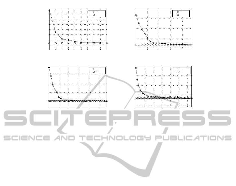
1 5 9 13 17 20

100

150

200

250

Optimal Solutions for V = 20

1 2 3 4 5 6 7 8 9 10

120

140

160

180

200

220

240

260

Optimal Solutions for V = 10

1 6 11 16 21 26 30

100

150

200

250

Optimal Solutions for V = 30

1 7 13 19 25 31 37 40

100

150

200

250

Optimal Solutions for V = 40

Figure 2: Optimal solutions for the star MILP when incrementing P .

the objective function values of the tree and star con-

ﬁgurations is not so large and that VNS improved the

solutions obtained with the star conﬁguration in most

of the cases, although, at a higher computational cost.

Finally, we observed that only a few nodes acting as

star nodes are required to obtain low energy levels

rapidly at the cost of low ﬂooding levels as well.

REFERENCES

Cormen, T., Leiserson, C., Rivest, R., and Stein, C. (2001).

Introduction to algorithms, second edition. MIT Press

and McGraw-Hill.

Elias, J. and Mehaoua, A. (2012). Energy-aware topology

design for wireless body area networks. In IEEE Inter-

national Conference on Communications, ICC 2012,

pages 3409–3410.

Fang, G. and Dutkiewicz, E. (2009). Bodymac: Energy

efﬁcient tdma-based mac protocol for wireless body

area networks. In 9th International Symposium on

Communications and Information Technology, ISCIT

2009, pages 1455–1459.

Glover, F. and Kochenberger, G. A. (2003). Handbook

in metaheuristics. International Series in Operations

Research and Management Science, Kluver Academic

Publishers, Springer 2003, 57:556.

Hansen, P. and Mladenovic, N. (2001). Variable neighbor-

hood search: Principles and applications. European

Journal of Operational Research, 130:449–467.

Huang, C., Liu, M., and Cheng, S. (2010). Wrap: A

weighted random value protocol for multiuser wire-

les body area networks. In IEEE International Sym-

posium On Spread Spectrum Techniques and Applica-

tions, ISSSTA 2010.

Kinsella, K. and Phillips, D. (2005). Global aging. The

challenge of success, Population Bulletin, 60.

Kwak, K. S., Ameen, M. A., Kwak, D., and Lee, C. (2009).

A study on proposed ieee 802.15 wban mac protocols.

In 9th International Symposium on Communications

and Information Technology, ISCIT 2009, pages 834–

840.

Pataki, G. (2003). Teaching integer programming formu-

lations using the traveling salesman problem. SIAM

REVIEW, 45(1):116–123.

Reusens, E., Wout, J., Latre, B., Braem, B., Vermeeren, G.,

Tanghe, E., Martens, L., Moerman, I., and Blondia,

C. (2009). Characterization of on-body communica-

tion channel and energy efﬁcient topology design for

wireless body area networks. IEEE Transactions on

Information Technology in Biomedicine, 13(6).

Ullah, S., Higgins, H., Braem, B., Latre, B., Blondia, C.,

Moerman, I., Saleem, S., Rahman, Z., and Kwak,

K. S. (2012). A comprehensive survey of wireless

body area networks on phy, mac, and network layers

solutions. Journal of Medical Systems, 36:1065–1094.

Yannakakis, M. (1991). Expressing combinatorial opti-

mization problems by linear programs. J. Comput.

Syst. Sci., 43(3):441–466.

ICORES2015-InternationalConferenceonOperationsResearchandEnterpriseSystems

132