A Decomposition Method for Frequency Assignment in Multibeam

Satellite Systems

Jean-Thomas Camino

1,2,3

, Christian Artigues

2,3

, Laurent Houssin

2,4

and Ste´phane Mourgues

Airbus Defence and Space, Space Systems, Telecommunication Systems Department,

31 Rue des Cosmonautes, 31402

Toulouse, France

CNRS, LAAS, 7 Avenue du Colonel Roche, F-31400 Toulouse, France

Univ de Toulouse, LAAS, F-31400 Toulouse, France

Univ de Toulouse, UPS, LAAS, F-31400 Toulouse, France

Keywords: Frequency Assignment, Multiprocessor Scheduling, Path Cover, Linear Programming, Constraint Program-

ming, Maximal Cliques Enumeration.

Abstract: To comply with the continually growing demand for multimedia content and higher throughputs, the telecom-

munication industry has to keep improving the use of the bandwidth resources, leading to the well-known

Frequency Assignment Problems (FAP). In this article, we present a new extension of these problems to the

case of satellite systems that use a multibeam coverage. With the models we propose, we make sure that for

each frequency plan produced there exists a corresponding satellite payload architecture that is cost-efficient

and decently complex. Two approaches are presented and compared : a global constraint program that handles

all the constraints simultaneously, and a decomposition method that involves both constraint programming

and integer linear programming. For the latter approach, we show that the two identified subproblems can re-

spectively be modeled as a multiprocessor scheduling problem and a path-covering problem, and this analogy

is used to prove that they both belong to the category of NP-hard problems. We also show that, for the most

common class of interference graphs in multibeam satellite systems, the maximal cliques can all be enumer-

ated in polynomial time and their number is relatively low, therefore it is perfectly acceptable to rely on them

in the scheduling model that we derived. Our experiments on realistic scenarios show that the decomposition

method proposed can indeed provide a solution of the problem when the global CP model does not.

1 INTRODUCTION

A common characteristic of any telecommunication

system is that it is bandwidth limited, and one of the

main challenges for the system engineers is to

optimally use this precious resource. Satellite

telecommunications systems are no exception to that

rule, and

this already difficult task is even more

complex when

the specific limitations and needs of

the satellite payload are taken into consideration.

Plenty of literature

can be found on the problem of

assigning frequencies under the name of “Frequency

Assignment Probems” (FAP). For instance, (Aardal

et al., 2007) is

a very thorough survey on the models

and the optimization methods that have been

developed over the

years to solve the frequency

assignment problems that

emerged in a lot of different

wireless communications

systems. The recent

litterature proposes more and

more sophisticated

methods to solve the FAP, such as parallel

hyperheuristics (Segura et al., 2011), differential

evolution (Salma et al., 2010), population-based

heuristics (Luna et al., 2011) (Yang et al.,

2014)

or considers more and more realistic variants of

the

FAP according to specific problem characteristics

(Koster and Tieves, 2012) (Muoz, 2012) (Wang and

Cai, 2014). This article aims at presenting new

models and approaches for this extension of the

frequency

assignment problem to multibeam satellite

systems,

and promising results on realistic scenarios.

A multibeam satellite system is characterized by

a plurality of relatively narrow beams used to provide

coverage to its service area as shown in Fig.1, each

beam being the representation of an antenna gain loss

threshold for the corresponding satellite radio source.

Still in Fig.1, the role of the satellite payload (2) is

to receive, downconvert, amplify, and retransmit the

signals of the uplink (1) in the different beams of the

Camino J., Artigues C., Houssin L. and Mourgues S..

A Decomposition Method for Frequency Assignment in Multibeam Satellite Systems .

DOI: 10.5220/0005218700230033

In Proceedings of the International Conference on Operations Research and Enterprise Systems (ICORES-2015), pages 23-33

ISBN: 978-989-758-075-8

 2015 SCITEPRESS (Science and Technology Publications, Lda.)

Figure 1: The uplink (1), the satellite payload (2) and the

downlink (3) of the forward link of a multibeam satellite

system.

downlink (3) where the end-users are located. It is

assumed that the system bandwidth is divided into

identical frequency channels, the bandwidth of a

channel

being equal to that of one carrier signal.

For each

beam, it is either specified by the operator or

assessed

in advance how much bandwidth is needed

and there-

fore how many carriers must be transmitted

in it. Assuming that the carrier uplink frequencies are

known

or treated afterwards, system engineers have to

define

for each carrier of each beam:

The frequency channel used in the downlink

The polarization of the signal in the downlink

The high power amplifier in the payload that will

be amplifying the corresponding uplink carrier

These are the variables of the problem presented

this paper. Values must be assigned to them with

the

goal to minimize the levels of interferences in

each

beam, the number of high power amplifiers

needed

in the satellite payload, and the number of

hardware

needed for the downconversions. More

precisely, the

approach we have selected is to aim

at minimizing

the number of high power amplifiers

needed in the

satellite payload since they are heavy,

expensive, and

highly power-consuming, while we

will be using

constraints to limit the interferences and

the hardware

needed for the downconversions to what

is acceptable.

The rest of the article is structured as follows. In

section 2, the problem constraints are listed and

detailed. Then, section 3 focuses on the different

approaches we have devised to actually model the

problem. Finally, section 4 provides experimental

results

and concrete scenario examples, before some

concluding remarks in section 5.

2 THE PROBLEM CONSTRAINTS

2.1

Frequency

Constraints

For the quality of transmission of a signal, the

interferences are a determining factor and any

frequency

assignment procedure should try to

minimize them.

Let us remind that a frequency and a

polarization must

be assigned to each carrier of each

beam in the downlink. Note that in this work, the

isolation of the signals

through the time-dimension is

not considered. In the

end, the frequency related

constraints that are taken

into account here are the

following :

Polarization Isolation:

A perfect radio antenna transmits and receives

waves in a particular polarization and is

insensitive to orthogonally polarized signals

(Bousquet

and Maral, 2009), meaning that the

same frequency channel can therefore be used

twice in the

same area without risking severe

interferences. In

actual facts, antennas cannot

transmit and receive

perfectly in one

polarization only, it is always a

combination of

two orthogonal polarizations, one

of them being

predominant. To take advantage of

that property

anyway, the choice here has been to

consider

that two carriers at the same frequency

using

orthogonal polarizations are allowed to be

transmitted in closer zones than two carriers

trans-

mitted at the same frequency and with

the same

polarization.

Spatial Isolation:

Thanks to antenna gain losses, two carriers can

use the same color (frequency or frequency-

polarization couple) as long as the two

corresponding beams are sufficiently distant

from each

other. This is often turned into a

constraint of

minimum distance between them,

leading the very

classic binary interference

constraints. The resulting representation is a

graph G

(B, E) where each vertex b

∈

corresponds to the zone covered

by a beam and

each edge e

∈

E is a link between two zones

where it is not allowed to use the same

color.

Limit on the Frequency Channel Reuse

Values:

Defining an upper-bound for these values

allows

to balance the number of times each

channel is

used, which reduces the hardware

needs for frequency conversions. Since two

uplink carriers can

only share a downconverter

ICORES2015-InternationalConferenceonOperationsResearchandEnterpriseSystems

in the satellite payload if they need the same

frequency downconversion, it is interesting to be

able to define the uplink

frequencies so as to

have as many of these situations as possible, and

this balance of the frequency reuse factors in the

downlink is advantageous on

that regard.

2.2 Amplification of the Signals

Constraints

A traveling-wave tube (TWT) is a type of high power

amplifier for radio frequency signals and a widely

used technology for satellite telecommunication

payloads (Bousquet and Maral, 2009). A TWT must

assigned to each carrier of each beam under the

following constraints:

Minimization of the Number of TWT:

A TWT is an expensive technology, one should

therefore aim at finding a distribution of the

carriers in the TWTs that minimizes their

number.

Frequency Ranges:

The TWTs can have a bandwidth narrower than

the overall system bandwidth. In that case, pay-

load engineers agree with the equipment

manufacturer on a limited number of frequency

ranges.

Therefore, the assignment of carriers to

the TWTs

must guarantee that the frequency

ranges are supported by the available equipment.

Carriers forbidden to use the same TWT:

Two carriers cannot be amplified by the same

TWT if their amplification requirements are too

different, because of the non-linearity of the

TWT.

These incompatibilities are known in

advance.

Single Use of the Frequency Channels:

A TWT cannot amplify two carriers using the

same frequency channel.

Limited Number of Carriers per TWT:

A TWT is characterized by its output power

level.

That power is shared by the carriers,

therefore the

number of carriers per TWT is

upper-bounded.

Contiguity of the Frequencies:

The payload complexity is assumed to be

significantly reduced when there are no

frequency gaps

between the carriers in the same

TWT.

3 MODELS

The first model we derived is a global constraint

program (section 3.1) that includes all the

aforementioned constraints. It has been able to

provide really interesting system solutions on some

scenarios, however, when the number of variables is

set to high realistic values, the global CP model fails

at providing solutions or proving unfeasibility in

reasonable time. That is why a decomposition

method has been developed, with a subdivision of

the problem

into a multiprocessor scheduling

(section 3.2) and a

path-covering (section 3.3)

problems. The two approaches, the single constraint

programming model

and the combination of the two

submodels, are then

compared experimentally in

section 4.

3.1 Global Constraint Programming

Model

The idea to derive a constraint programming model

has been motivated by an analysis of the constraints

on the problem variables (frequency, polarization,

TWT) that revealed that global constraints could be

used to model a large part of the problem. A global

constraint (Beldiceanu et al., 2005) is a set of con-

straints for which it is preferable to treat that set of

constraints as a whole than to treat all the constraints

of that conjunction of constraints individually. Using

global constraints is a way to have a better view on

the structure of the problem, which is then exploited

with powerful filtering algorithms. On that regard, a

very significant example is the all different constraint

(van Hoeve, 2001)

alldifferent(X )

that forces all the variables of the array X to be

different. In the model below, we also use the global

cardinality constraint

global_cardinality_constr(X ,Y ,m,M)

that allows to bound the number of times some items

appear in a list, X being that list, Y the set of sought

values, m the array of minimum number of

occurrences for each sought value, M the array of

maximum number of occurrences for each sought

value. Finally, the Gecode convexity global constraint

convex(X )

is used to force the integers of an integer set X to be

a convex sequence ({1, 2, 3} is one while {1, 2, 4} is

not). These global constraints are implemented in the

open source solver Gecode (Schulte et al., 2013) that

we chose to use.

ADecompositionMethodforFrequencyAssignmentinMultibeamSatelliteSystems

An instance of this particular frequency

assignment problem is defined by a set of N

beams,

each beam b

∈

{1, · · · , N

} being characterized by

the number n

of carriers transmitted in it, leading to

an overall number of carriers















For all

∈

and for all

∈

{

, · · · , n

}

ind



,

















defines a 1D sorting of these carriers and for all

∈

{ind(

b, c

)

∈

, · · · , n

}}

is the notation for the set of indices of the carriers of

the b

beam. Therefore, note that the C

sets

partition the set C

{1, · · · , N

}. The system

bandwidth is divided into N

sub-channels indexed

by F

{1, · · · , N

}. N

TWTs are available in the

payload, and N

orthogonal polarizations are

considered

(typically

2), the corresponding

index sets be

ing respectively denoted by T and P.

Each carrier

∈

C must be assigned a frequency

channel f

∈

F ,

a TWT t

∈

T and a polarization

∈ P. These are

the problem variables. Two graphs

(

B, E

) and

G′

(B, E′) with E′

⊂

E are defined:

an edge of E′ forbids the carriers in the two

corresponding beams to use the same frequency

channel whatever the polarization, whereas an edge

of E only forbids the multiple use of the same

frequency-polarization couple.

In the following

equations, note that card(X ) denotes

the cardinality of

the set X . Here follows the list of

the constraints

expressed with these variables:

For a given beam b such that n

> 1, the n

carriers must be contiguous in frequency, use the

same

TWT, and have the same polarization. For

such b

values, the constraints are:

∀

∈ {

· · ·

, n

}

ind(

b,i

)

ind(

b,i

)

ind(

b,i



ind(

b,i

)



)

As discussed in section 2.1, channel reuse

bounds

are a tunable parameter in input used to

limit hardware needs for the downconversions.

Let R

min

and R

max

be the arrays of size N

these bounds

(note that in practice the lower-

bound array is set

to 0, it is just there to fit the

definition of the global

constraint that use both

arrays), then the corresponding corresponding

is the following:

global_ cardinality_constr(f, F, R

min

, R

max

)

The binary interference constraints associated

to E can be expressed as follows for all b, b′

∈

such that b < b′ and (b, b′)

∈

E :

alldifferent (f

 1)

c ∈ C

∪ C

ʼ)

)

And for E′, for all b, b′

∈

B such that b < b′ and

(

b, b

′

)

∈

′

alldifferent

(

∈

∪

b’

)

The same frequency cannot be used twice by the

carriers of a given TWT :

∀

∈

∀

∈

card(

∩

)

≤

)

where T

⊂

C and F

⊂

C respectively are the set

of carriers using the TWT t and the set of carriers

using the frequency channel f , these set variables

being linked to the arrays t and f by side

channeling constraints that we do not provide

here for the

sake of conciseness.

The contiguity in the TWTs. Let us denote by F

the set of frequency channels used in the TWT

these set variables being easily defined with

chan-

neling constraints involving the variable

arrays f

and t. Then, the global constraint convex

does exactly what is sought:

∀

∈

convex(

)

The maximum number of carriers in a given

TWT

that is upper bounded by a tunable

parameter n :

∀

∈

card(

)

≤

)

The incompatibilities between the carriers that

cannot use the same TWT. Let c, c’

∈

C be two

carriers forbidden to use the same TWT, then the

corresponding constraint is the following:



′

(10

)

The content of the TWTs must be of a given type.

Let F

⊂

F and F

⊂

F be two subparts of the

system bandwidth such that F

∪

F. These

two sets define two types of acceptable frequency

contents for the TWTs, which means that the

carriers

in a given TWT must either all be in F

or all be

in F

, which can be expressed as

follows:

∀

c, c

′

∈

F\F

∧

c’

∈

F\F

⇒



′

(11

)

The objective is the minimization of the number

available TWTs actually used. That number n

used

ICORES2015-InternationalConferenceonOperationsResearchandEnterpriseSystems

a variable that can be obtained from the array t

with

two successive global counting constraints, the

first

one generating an array of the number of times

each

TWT is used, the second counting the number of

non-

zero values in the latter:

min n

used

(12

)

3.2 Multiprocessor Scheduling Part

3.2.1 The Scheduling Model

An analogy with multiprocessor scheduling problems

is possible for the assignment of frequencies and

polarizations, that is for the subproblem that only

concerns the variable arrays f, p, and the constraints

(2), (3), (4), (5) and (6). That problem, denoted by

), is an extension of the model proposed in

(Kiatmanaroj et al., 2013) where the frequency

assignment is addressed regardless of the

polarizations. Each beam b

∈

B is assimilated to a

single operation job whose processing time,

expressed in time units, is non-preemptive and equal

the number of carriers in that beam. Note that such

a model is only

valid because the frequencies of the

carriers in a same

beam are constrained by constraint

(8) to be contiguous, the contiguousness of

frequencies corresponding therefore to the non-

preemptiveness of the processing times. Each

maximal clique of G′ is assimilated to a machine with

non-overlapping constraints,

while each maximal

clique of G is associated to exactly two machines,

one for each polarization. For each beam/job b

∈

B ,

C′

denotes the set of machines that correspond to the

cliques of G′ that contain b, while C

b,1

and C

b,2

are

the sets of machines representing the cliques of G

containing b that are respectively

associated to the

polarizations 1 and 2. For constraint

(4), it is assumed

that the only restriction here is an upper-bound on

the reuse factor R

∈

of the channels (same bound

for each channel), which leads to

the definition of

, · · · , m

} identical parallel machines. Each

job b

∈

B requires simultaneously multiple machines.

More precisely, it must be executed on:

all the machines of

C’

either all the machines of C

b,1

, or all the machines

of C

b,2

one machine of M

Note that relying on cliques is not necessary to make

this analogy with multiprocessor scheduling, another

option could be to define a machine for each binary

constraint, but relying on cliques allows to take into

account several constraints simultaneously, just like

global constraints in constraint programming. In the

example of Fig.2, for the beam number 1 with the

notations

′







,

,



,

,

,



,,

,

,,



and



,



,,

,

,,



, we have:

′

,

and ′

,

associated to the cliques/machines

{1,2} and {1,3} of G’



,,

and 

,,

associated to the machines of first

polarization for the cliques {1,2,3} and {1,3,4}

in G



,,

and 

,,

associated to the machines of

second polarization for the cliques {1,2,3} and

{1,3,4} in G





the machine M used by the beam 1

In the example, the two carriers required in beam

1 use the second and third frequency channels and

the first kind of polarization. With a common

deadline for all the jobs being equal to the number of

frequency channels N

(equal to 4 in Fig.2), one can

see that solving this scheduling problem is equivalent

to solving the considered subpart of our frequency

assignment problem.

Figure 2: Example of execution of one job on the

machines.

Proposition: (S

) is equivalent to solving a

multiprocessor scheduling problem, it is

therefore

NP-hard.

Proof: The parallel machine problem is a par-

ticular case of (S

3.2.2 Maximal Cliques Enumeration in

Multibeam Satellites Interference

Graphs

As explained in the previous paragraph, one

promising direction to solve efficiently the

scheduling part of the frequency assignment problem



ADecompositionMethodforFrequencyAssignmentinMultibeamSatelliteSystems

considered is to use the cliques of the interference

graphs. It is thus of interest to study the theoretical

and practical complexity of enumerating the maximal

cliques. In multibeam systems, the analysis of their

exhaustive enumeration differs depending on the type

of graphs considered: regular layouts or random

interference graphs.

Cliques in Regular Layouts

A regular layout is an organization of the beams that

provides a continuous coverage of the zone with

overlapping beams that describe an hexagonal lattice,

as shown in Fig.1 for instance. It is a very common

choice for the system engineer since the contiguous

coverage it provides can be a crucial specification of

the customer, and also, it requires simpler antenna

designs than a non-uniform layout. For a beam b

∈

let us denote by

the position of its center and by

Γ(b) the set of its adjacent beams. A common

industrial approach for a regular layout with beams of

radius r is have Γ(b)

= {

∈

≠ b and || c

− c

||<d}

with d being equal to either 3r or 2

√

r leading to the

representations (a) and (c) of Fig.3. They are usually

called 3-colors pattern and 4-colors pattern because

with such edges in the interference graph, it is

possible to partition the set of vertices into

respectively 3 and 4 independent sets as shown in

figure (b) and (d) of Fig.3. An important property of

the regular interference graphs with the edges defined

this way is the following:

(a)

(b)



Figure 3: (a) Adjacent beams, 3r threshold (b) Independent

sets, 3r threshold (c) Adjacent beams, 2

√

r threshold (d)

Independent sets, 2

√

r threshold.

Proposition: The maximal cliques of the

interference graphs corresponding to the regular

patterns

in regular layouts can all be enumerated in

polynomial time

Proof: The key idea is that for each exclusion

pattern, there exists a finite number m such that for

each vertex b

∈

B there exist m potential cliques that

might contain b, m being independent of the size N

of the graph. For instance, for a graph with the edges

of the 4-colors pattern, geometrical considerations

allow to understand that, for a given vertex :

it cannot belong to a clique of size 5 and more,

the cliques of size 4 that might contain it are

those of Fig.4 plus those obtained by rotating of





around the center of the corresponding beam

leading to a total of 20 distinct potential cliques,

the only way it can belong to a maximal clique

of size 1, 2 or 3 is that the corresponding beam

surrounded by less beams than in the full

configuration of Fig.4, which can happen either

because

the beam in question is near the bound

of the layout or because there are “holes” in it.

Therefore, if such a clique exists, it is a

subgraph of what

would have been a clique of

size 4 if some beams

had not been missing.

These situations are also in

finite number and can

be precisely enumerated.

Figure 4: Cliques of size 4 with 4-colors pattern.

Note that in the example of the 4-colors pattern, the

number of cliques is therefore upper-bounded by

20N

. Each potential clique is characterized by a

specific set of adjacent beams and, for the cliques of

size less than 4, a set of non-existing beams whose

positions are perfectly known in terms of distance to

the beam tested and orientation with respect to a given

reference direction, say the horizontal direction. The

same type of rationale applies for the graphs defined

with the 3-colors pattern. Therefore, to enumerate all

the maximal cliques in the case of regular layouts, one

would only have to iterate on the vertices b

∈

B, that

is on the beams, and test each clique possibility to

see which ones actually exist for each b. That way,

the list of maximal cliques can gradually grow,

simple tests allowing to avoid redundancies. In the

end, the maximal cliques of the regular layouts are

indeed

enumerated with a polynomial complexity.

ICORES2015-InternationalConferenceonOperationsResearchandEnterpriseSystems

Cliques in Realistic Random Layouts

Even if the standard way to design a layout is to rely

on the uniform patterns, it can be interesting to break

that regularity in order to match the heterogeneity of

the requirements over the service area. One can there-

fore have to work with a layout that can have beams

of differents widths and positions for their centers that

do not describe any particular known geometrical

pattern. It was therefore necessary in that case

determine whether it was still an acceptable

approach to enumerate the cliques before actually

solving the frequency assignment problem. To do

so,

the slightly modified version of the Bron-

Kerbosch

(Bron and Kerbosch, 1973) algorithm

proposed by

Tomita et al. (Tomita et al., 2006) has

been implemented and used on sets of graphs that were

randomly

generated with constraints on the vertex

degrees. In

practice, in multibeam satellite systems

interference

graphs, these vertex degrees are rarely

less than 1 and

greater than 12, so this has been

specified as the main

constraint in the constraint

program used to generate

these graphs. We generated

10000 different graphs of size |B]

200 (maximum

size for a realistic scenario) and observed that the

mean number of cliques was 881 and the mean

execution time was 14 millisec-

onds. These cliques

numbers are far from the 3





upper bound of the

number of cliques in an undirected

graph, which is

very interesting in practice because

too high numbers

of cliques could have made it impossible or

unreasonable to rely on a model based on

them. But

most importantly, the computational times

are

relatively low, even instantaneous at the time scale

the designing phases of the satellite

telecommunication systems. In the end, this means

that this preliminary enumeration of the cliques is a

pre-processing

operation for the frequency

assignment problem that

is perfectly acceptable,

whatever the type of layout.

3.3 Path Covering Part

Let us assume that the frequencies and the

polarizations have been assigned somehow to the

carriers

of a given system, possibly with a scheduling

based

procedure as the one presented in section 3.2.

Then,

one can wonder what the problem of

assigning the

TWTs to these carriers becomes, that

problem being

denoted by (S

). The first important

remark is that

the constraint 11 on the type of TWTs

can now be

seen as additional incompatibilities in

constraint 10

since the frequencies of the carriers are

now known.

The second is that it is now possible to

represent the

problem as a path-covering problem of

a digraph in

which the vertices represent the N

carriers of the

system (see Fig. 5), a path

representing a TWT and its content. In this graph,

for all f

∈

F\{N

}, the only possible direct successors

of the carriers using the frequency f are those using

the frequency f

the in-degrees of the carriers

using the frequency 1

being all equal to 0, just like

the out-degrees of the

carriers using the frequency

. As a consequence

of these few properties, such

graphs are acyclic. The

incompatibilities between

two carriers that cannot

be in the same TWT/path

are represented with

dotted-line connections. For a

given carrier, two

situations impact the number of

out-arcs : when this

carrier is not the last carrier of the

beam it belongs to,

and when there exist

incompatible carriers that use

the next frequency. In

the former case, only one arc

leaves the carrier

considered and its head is the next carrier in the

Figure 5: Carrier based graph for TWT assignment.

corresponding beam. In the latter case,

the carrier

cannot be connected to the carriers with

which an

incompatibility is shared. Otherwise, for a

carrier

that is not in any of these two situations, it is

connected to all the carriers using the next frequency.

One can then see that assigning TWTs to the carriers

comes down in that case to finding the minimum

number of disjoint paths that cover all the vertices,

the contiguity (constraint 8) and the fact that the same

frequency cannot be used twice in a TWT (constraint

7) being automatically verified with a graph built that

way. But there are also some additional constraints

to take into account such as the upper-bound for the

length of the paths (constraint 9), the constraint not

to use the same TWT for two incompatible carriers

(constraint 10), and finally the constraint that the

carriers of a block of carriers must use the same

TWT (constraint 1). In the end, an instance of the

problem considered is entirely defined by : an acyclic

digraph D whose vertices can be partitioned into a

certain number of ordered “levels” and whose arcs

are only between two vertices of a level and the next,

an upper bound l for the length of the paths, a set for

ADecompositionMethodforFrequencyAssignmentinMultibeamSatelliteSystems

each carrier of the carriers it must share a TWT with

(empty sets being allowed), and a set for each carrier

of the carriers incompatible with that carrier (empty

sets also allowed).

Proposition: (S

) is an NP-hard path-covering

problem

Proof: Without the additional constraints (1,9,10),

the problem of covering a digraph with a minimum

number of point-disjoint paths can be solved in

polynomial time as shown in (Boesch and Gimpel,

1977). But once they are taken into account, it can be

proven that the problem becomes NP-hard. Indeed,

let us consider an instance of the problem of finding

a minimum cardinality cover of the elements of a

partially ordered set (poset) with chains of restricted

length, whose NP-completeness has been proven in

(Shum and Trotter, 1996). It is common to represent

that poset with a digraph partitioned in ordered levels,

the edges connecting the comparable elements of

the set from one level to the next: this is precisely

Hasse diagram. Then, with the upper bound for

the

path lengths equal to the maximum length of a

chain

and with, for each carrier, empty sets for the

sets of

carriers that must use the same TWT and

the sets

of incompatible carriers, one can see that

solving

this poset cover instance is equivalent to

solving a

particular instance of the path-covering

problem

considered in this paper. Therefore, it is also

NP-

complete.

To solve it, the following integer linear

programming

model has been derived :











(13

)

s.t.

∀∈,



1







(14

)

∀∈,∀



∈,







1







(15

)

∀∈,



















(16

)

∀∈,











(17

)

∀,



∈that are incompatible, ∀∈,









1

(18

)

∀,



∈ in the same block of carriers ∀∈,













0

(19

)

∀∈,∀∈



,

 











































(20

)

where y

c f

∈

{0, 1} are input Boolean arguments that

indicate whether the carrier c

∈

C uses the frequency f

∈

F , x

{0, 1} are the Boolean variables that indicate

the carrier

∈

uses the TWT

∈

, and finally

the

∈

{0, 1} are the Boolean variables that indicate

whether the TWT t is actually used. Constraint 14 is

the constraint to have only one TWT assigned to each

carrier, 15 forbids a given TWT to be used by two

different carriers using the same frequency channel,

16 is the constraint that forces the u

to be equal to 1

soon as the TWT t is used at least once, 17 is the

limit

on the number of carriers in the same TWT,

constraint

18 forbids two incompatible carriers to use

the same

TWT, 19 forces the carriers in the same block

of carriers to use the same TWT, 20 ensures the

contiguity of

the frequency channels in each TWT,

finally 13 is the

minimization of the number of TWT

actually used.

4 EXPERIMENTAL RESULTS

Experiments were needed to assess the performances

of the two following approaches:

Global Approach (GA):

The global constraint program of section 3.1

solved with a CP solver (Gecode)

Decomposition Method (DM) :

Sequential solving of (S

) of section 3.2 with

CP solver (Gecode) and then of (S

) of

section 3.3 with an ILP solver (Gurobi)

A first detailed example is presented in Fig.6 with a

fictitious scenario over France and Italy, with N

regularly organized beams. The characteristics of the

problem solved were the following :

Each beam

∈

{

, · · · ,

}

of Fig.6 has a required

number of carriers n

than is either equal to 1 or

to 2, the carriers being indexed as shown inside

the beams in Fig.6a

ICORES2015-InternationalConferenceonOperationsResearchandEnterpriseSystems

For the beams b with a number of carriers

>1,

we require contiguous carrier

frequencies, same

polarization and same TWT

The system bandwidth is divided into

channels

The acceptable frequency ranges for the

TWTs

are {1, 2, 3} and {4, 5, 6}

The TWT reuse upper-bound is set to 3, i.e.

the width of an admissible frequency range

The 4-color pattern is used to define binary

interference constraints for the reuse of the

same

frequency-polarization couple (Fig.3c)

The 3-color pattern is used to define binary

interference constraints for the reuse of the

same frequency, regardless of the polarization

(Fig.3a)

Carrier n◦5 is incompatible with carriers n◦9

and n◦10, carrier n◦13 is incompatible with

carriers n◦17 and n◦18, carrier n◦7 is

incompatible with n◦8, which means that they

cannot use the same TWT

Each frequency channel must be used at

most

third times

Objective function : number of TWTs used

(a)

(b)

Figure 6: (a) Multibeam coverage and polarizations (b)

Frequencies and TWTs.

This is one of the instances for which GA

solved

with Gecode is unacceptably long to find a

solution.

On the other hand, with DM, the scheduling

part and

the subsequent binary linear program are

both solved

extremely efficiently respectively by

Gecode and

Gurobi. On Fig.6a, the regular layout is

reprensented

with a ring color for each polarization,

and on Fig.6b,

the frequencies of the carriers found in

the scheduling

part can be read on the horizontal axis,

and each color

for the carriers represents one TWT.

Note that the

design of Fig.6 obtained for that

example is optimal

since the number of TWTs used

is exactly equal

to the number of carriers divided

by the maximum

number of carriers in a TWT.

When instances are randomly generated, note

that

there is no guarantee that they will be feasible.

Even

if this is true for both approaches, in the case of

DM,

this risk of infeasibility is even increased since

some

of the path-covering problem constraints are

currently not anticipated in the preceding scheduling

problem (the frequency ranges of the TWTs for

instance). In practice, infeasibility is significantly

harder to detect than actual solutions for feasible

instances, at least when Gecode is used, that is in GA

and in (S

) of DM. In the results of this section, the

statistic values presented only consider the instances

that turned out to be feasible.

For each instance tested with the DM approach,

the

corresponding (S

) scheduling problem is solved

with Gecode using the corresponding subset of

constraints in the global model of section 3.1. Then,

the solutions of (S

) are transformed into (S

)

path-

covering instances that are solved with Gurobi

thanks to the ILP model we derived in section 3.3.

With GA, let us remind that the problem is entirely

solved with Gecode. For the first phase of our series

of experiments, we generated FAP instances with

similar characteristics as the example detailed before,

with the following few changes :

Each beam b

∈

{1, · · · , 12} of Fig.6 has a now

required number of carriers n

than is either

equal to 0 or to 1

The TWT carrier incompatibilities are now

ran-

domly generated (about 10% of all the

possible

carrier couples)

The overall number of required carriers

∑





is gradually increased, from

4 to 12, 100 feasible instances being generated

at each stage

Each frequency channel cannot be used more

than

once when 4 ≤ N

≤ 6 and more than twice

when

7 ≤ N

≤ 12

ADecompositionMethodforFrequencyAssignmentinMultibeamSatelliteSystems

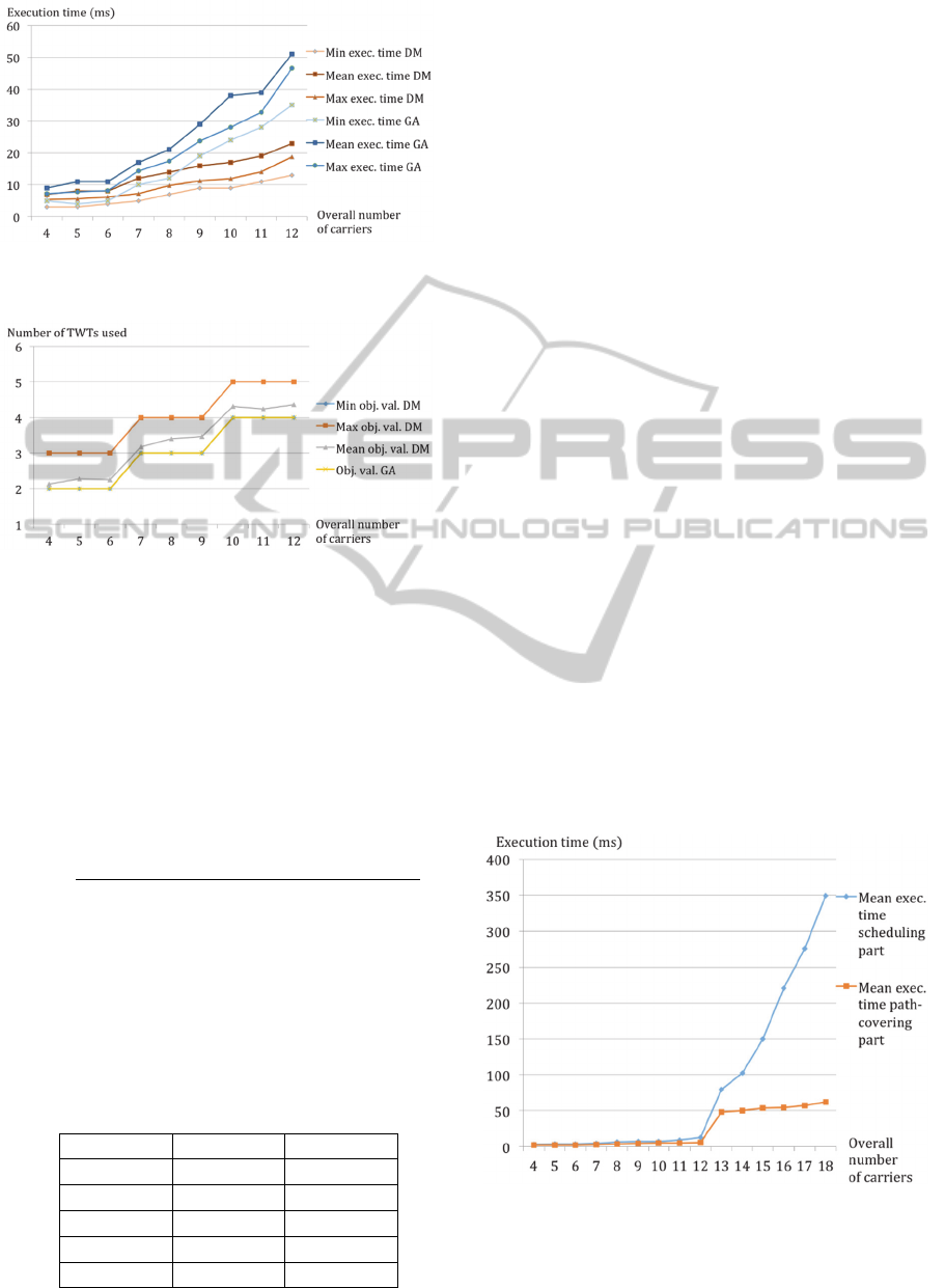
Figure 7: Comparison of GA and DM on 4-carriers to 12-

carriers instances with execution time statistics.

Figure 8: Comparison of GA and DM on 4-carriers to 12-

carriers instances with objective value statistics.

Fig. 8 and Fig. 7 allow to compare GA and DM

terms of objective values and execution times. As

expected, we can observe that in the the case of a

joint assignment of TWT, frequency and polarization

to the carriers (GA), the execution times are greater

than those of DM but the objective values are better

in average. In the particular case of the instances we

generated, GA always reaches the theoretical optimal

value which is equal to

ceiling

Overallnumberofcarriers

MaximumnumberofcarriersinaTWT



However, the decomposition method often manages

to reach that optimal number of TWTs too as shown

in Table 1. This is a crucial remark we wanted to

emphasize since it is what legitimates the use of DM

when GA is not usable in practice.

Table 1: Percentage of times the theoretical optimum is

reached with DM for each set of instances of varying num-

ber of carriers.

4 carriers 5 carriers 6 carriers

87% 72% 75%

7 carriers 8 carriers 9 carriers

83% 59% 53%

10 carriers 11 carriers 12 carriers

69% 76% 64%

In the next phase of our experiments, the overall

number of carriers in the system has been set to be

greater

than 12 and less than 19, the carrier

requirements in

each beam being either equal to 1 or

2, and the frequency channel reuse limit being now

set to 3. As a

result, some new constraints have to be

taken into account for the beams b such that n

> 1 :

contiguity of

frequencies, same polarization and same

TWT for the

carriers belonging to the same beam. In

practice, this

is the point where GA becomes unusable

both for feasible and infeasible instances, because of

extremely

long execution times even on these

instances that are

still relatively small compared to the

biggest realistic

situations. This explains why it has

been necessary to

develop DM. In Fig. 9, the

execution times of (S

)

(scheduling) and (S

) (path-

covering) are compared

on the whole range of

instances, from 4-carriers instances to 18-carriers

instances. Two main things can

be observed in that

figure. First, the difference between the instances

with at most 12 carriers and those

with at least 13

carriers is clear: the new constraints

linked to the

beams for which the carrier requirement

is strictly

higher than one slow the search. Also, we

see that

the computational times grow faster for the

scheduling problem than for the path-covering

problem. That remark is even more important when

we consider the fact that infeasible instances are also

re-

ally hard to detect for Gecode in the scheduling

part.

) is therefore the subproblem that deserves

attention for future work, the goal being to

solve the

highest realistic instances. Our not yet

exploited analysis of the cliques in the interference

graphs could

certainly be an interesting direction.

Figure 9: (S

) (scheduling part) and (S

) (path-covering

part) execution times.

ICORES2015-InternationalConferenceonOperationsResearchandEnterpriseSystems

5 CONCLUSION

The models we proposed for this particular frequency

assignment problem applied to the design of multi-

beam satellite systems allowed to algorithmically

solve instances that could not be solved by satellite

telecommunications engineers. We showed that the

decomposition method we devised could produce so-

lutions and even optimal solutions in reasonable

computational times especially compared to the

perfor-

mances of the global constraint program for

that prob-

lem. We also showed that relying on the

cliques of

the interference graphs was an acceptable

direction

and most likely a way to improve our

current algorithms for the scheduling subproblem of

our decomposition method. Concerning the path-

covering problem, a series of experiments showed

that realistic instances where solved almost

instantaneously by the

solver Gurobi, which tells us

that we extracted an

interesting subproblem, and we

will definitely try to

take advantage of this in some

way in the next algorithms we will implement. To

solve the largest realistic instances, work still has to be

done to get faster results and improving the algorithms

for the scheduling

part might not be enough. Instead

of solving the two

identified subproblems

sequentially, we might aim at more integrated

approaches inspired by combinatorial

Benders’ cuts

for instance, or with filtering algorithms

solving

locally the path covering problem.

REFERENCES

Aardal, K. I., van Hoesel, S. P. M., Koster, A. M. C. A.,

Mannino, C., and Sassano, A. (2007). Models and so-

lution techniques for frequency assignment problems.

Annals of Operations Research, 153:79–129.

Beldiceanu, N., Carlsson, M., and Rampon, J.-X. (2005).

Global constraint catalog. SICS Research Report.

Boesch, F. T. and Gimpel, J. F. (1977). Covering the points

of a digraph with point-disjoint paths and its appli-

cation to code optimization. Journal of the ACM,

24:192–198.

Bousquet, M. and Maral, G. (2009). Satellite Communica-

tions Systems : Systems, Techniques and Technology.

edition.

Bron, C. and Kerbosch, J. (1973). Finding all cliques of

an undirected graph. Communications of the ACM,

16:575–577.

Kiatmanaroj, K., Artigues, C., and Houssin, L. (2013). On

scheduling models for the frequency interval assign-

ment problem with cumulative interferences.

Koster, A. and Tieves, M. (2012). Column generation for

frequency assignment in slow frequency hopping net-

works. EURASIP Journal on Wireless Communica-

tions and Networking, 2012(1):1–14.

Luna, F., Estbanez, C., Len, C., Chaves-Gonzlez, J., Nebro,

A., Aler, R., and Gmez-Pulido, J. (2011). Optimiza-

tion algorithms for large-scale real-world instances of

the frequency assignment problem. Soft Computing,

15(5):975–990.

Muoz, D. (2012). Algorithms for the generalized weighted

frequency assignment problem. Computers and Oper-

ations Research, 39(12):3256–3266.

Salma, A., Omran, I. A. M., and Mohammad, M. (2010).

Frequency assignment problem in satellite communi-

cations using differential evolution. Computers and

Operations Research, 37(12):2152–2163.

Schulte, C., Tack, G., and Lagerkvist, M. Z. (2013). Mod-

eling and programming with gecode. 522.

Segura, C., Miranda, G., and Len, C. (2011). Parallel hy-

perheuristics for the frequency assignment problem.

Memetic Computing, 3(1):33–49.

Shum, H. and Trotter, L. E. (1996). Cardinality-restricted

chains and antichains in partially ordered sets. Dis-

crete Applied Mathematics, pages 421–439.

Tomita, E., Tanaka, A., and Takahashi, H. (2006). The

worst-case time complexity for generating all maxi-

mal cliques and computational experiments. Theoret-

ical Computer Science, 363:28–42.

van Hoeve, W.-J. (2001). The alldifferent constraint: A sur-

vey. Cornell University Library.

Wang, J. and Cai, Y. (2014). Multiobjective evolutionary al-

gorithm for frequency assignment problem in satellite

communications. Soft Computing, pages 1–25.

Yang, C., Peng, S., Jiang, B., Wang, L., and Li, R.

(2014).

Hyper-heuristic genetic algorithm for solv-

ing

frequency assignment problem in td-scdma. In

Proceedings of the 2014 conference companion on

Genetic and evolutionary computation companion,

ACM:1231–1238.

ADecompositionMethodforFrequencyAssignmentinMultibeamSatelliteSystems