
Resource Allocation and Scheduling based on Emergent behaviours in
Multi-Agent Scenarios
Hanno Hildmann and Miquel Martin
NEC Laboratories Europe, Kurf¨ursten-Anlage 36, D-69115 Heidelberg, Germany
Keywords:
Resource Allocation, Scheduling, Emergence, Optimization, Stochastic Optimization, Routing, Logistics.
Abstract:
We present our observations regarding the emergent behaviour in a population of agents following a recently
presented nature inspired resource allocation / scheduling method. By having agents distribute tasks among
themselves based on their local view of the problem, we successfully balance the work across agents, while
remaining flexible to adapt to dynamic scenarios where tasks are added, removed or modified. We explain the
approach and within it the mechanisms that give rise to the emergent behaviour; we discuss the model used
for the simulations, outline the algorithm and provide results illustrating the performance of the method.
1 INTRODUCTION
Resource allocation, as discussed in (Luss, 2012), of
which scheduling is a prominent type, is a wide field
and applicable to a large number of commercial en-
deavors, e.g. (Pinedo, 2012). Many approaches to
this domain exist and it is not the goal of this paper to
compare between these, nor is it to champion one over
the other. The pervasive nature of the topic suggests
that different instances of the problem with a range of
attributes and challenges will make it unlikely for any
single approach to consistently outperform all others.
In this paper we would like to discuss one dis-
tributed resource allocation method (Hildmann and
Martin, 2014) and, specifically, the emergence of sim-
ple properties in a population of agents using this
method. Emergence is normally linked to the interac-
tion between members of a population, not to their in-
dividual actions (Holland, 1998); we discuss the inter-
action between agents, and investigate the effect this
has on the behaviour of the population as a whole.
The example problem we simulated to evaluate
the approach is a scheduling scenario. Application
of the method to civil security services like police or
fire fighters is currently considered, but for the run-
ning example in this paper we chose the utility sector
and the daily schedules of field service personnel.
We think the views presented in this paper are
of interest to the optimization community and to re-
search in Artificial / Swarm Intelligence; furthermore
we see applications in the areas of Transportation and
Scheduling (Dussutour et al., 2004).
2 PROBLEM DESCRIPTION
We simulated the dispatching of service personnel,
tasked with executing a number of tasks within their
shift. The time required to handle a task is predicted
in advance. In day to day operations traffic conditions
affect travel times between locations and, when arriv-
ing on site, a task might transpire to require less or
more time than originally predicted. The problem can
be stated as the sequential scheduling of service or
maintenance tasks for a group of field engineers, with
the cost of the schedule being calculated in terms of
the time it takes to process the schedule:
Description: Let A be a set of agents a
1
, . . . , a
m
, each
with a finite amount of resources r
a
i
as well as a depot
d
a
i
, let T be a set of tasks t
1
, . . . , t
n
each with a cost
c
t
j
and assume that function f(L × L ) → c
l1l2
maps
tuples of locations (for the agents or depots) to a cost.
The problem is then to allocate the tasks to agents
such that (a) all tasks are allocated to exactly one
agent and (b) the minimal sum of the cost to connect
the depot to all tasks allocated to this agent (i.e. the
shortest path) plus the sum of the costs of the tasks
themselves does not exceed the agent’s capacity.
The presented approachis designed to handle non-
static problems (Hildmann and Martin, 2014) and the
following 4 aspects are considered to be dynamic:
(1) A (agents may join the population or drop out),
(2) T (tasks may be added or removed),
(3) f() (tasks may change their location) and
(4) c
t
j
(tasks may change their cost).
140
Hildmann H. and Martin M..
Resource Allocation and Scheduling based on Emergent behaviours in Multi-Agent Scenarios.
DOI: 10.5220/0005219501400147
In Proceedings of the International Conference on Operations Research and Enterprise Systems (ICORES-2015), pages 140-147
ISBN: 978-989-758-075-8
Copyright
c
2015 SCITEPRESS (Science and Technology Publications, Lda.)

3 MODEL
The model simplifies the problem in the following
ways: the act of re-allocating a task from one agent to
another (stealing) is assumed to be instantaneous and
cost free. In each iteration, all agents are activated in
randomized order, and finally, agents have a starting
location (depot) and maintain individual schedules.
Parameters: The problem model has the following
parameters: numbers of both, agents and tasks, the ca-
pacity of each individual agent (which is the same for
all agents), the visibility range, the map size (we used
100 × 100 for all the simulations discussed in this pa-
per) and finally a flag determining whether a single
depot is used or whether there are multiple depots.
Furthermore, formula 1, given below, includes the
tuning parameter α. Changes in α will affect the
speed with which the approach converges towards a
stable state, and on the other hand, the degree of
change in the problem that the algorithm can handle.
Formulae: The decision to re-allocate a task from
the active agent A to the passive agent B is stochastic.
If agent A is balanced this probability (P
bal
A
) is:
P
bal
A
= 1−
(rem.cap
B
)
α
(rem.cap
A
)
α
+ (rem.cap
B
)
α
(1)
with rem.cap
X
the remaining capacity of X. The prob-
ability for a maximizing agent A (P
max
A
) is the inverse:
P
max
A
= 1− P
bal
A
(2)
4 METHOD, APPROACH AND
ALGORITHM
There is plenty of evidence (e.g. (Bartholdi and
Eisenstein, 1996)) for the potential of nature-inspired
scheduling to be extremely efficient; our work is in-
spired by the behavior of social insects (Camazine
et al., 2001). It is known (Bonabeau et al., 2000) that
colonies of social insects like bees, termites or ants
seem to operate in a semi-stable pattern until some
catalyzing event like e.g. the discovery of a new food
source or an attack on the colony takes place. This
then triggers a paradigm shift in the whole colony
which persists until the event is dealt with, after which
the system returns to the semi-stable state.
We present our work on 3 levels: the method, the
approach and the implemented algorithm. By method
we mean the generic description of how a population
of agents can cooperate to collectively cope with a
large number of tasks in dynamic environments. The
approach describes how this method can be applied in
computer science and to our example.
4.1 Method
Two opposing mechanisms govern the interaction be-
tween the agents: one to exchange tasks between
themselves with the aim to balance the length of their
respective schedules; and the other to re-schedule
tasks in order to largely reduce some agents’ loads.
Both mechanisms define interaction between ex-
actly two agents and in both cases the decision to
re-allocate a task is stochastic (using the formulae 1
and 2, respectively). The process is applied continu-
ously; converging towards balanced or highly unbal-
anced workloads. As the mechanisms are stochastic
they rely in a large number of interactions to achieve
their goals, but on the other hand facilitate the ability
to overcome deadlocks and local optima.
The first mechanism enforces a semi-stable equi-
table state where agents exchange tasks to maintain a
level of fairness: individual tasks can be moved from
one schedule to another if this decreases the differ-
ence in the respective agents’ loads.
The second mechanism, which differs only
marginally from the first, is used to achieve its ex-
act opposite: the re-allocation of tasks between two
agents is determined on the basis of whether the re-
allocation increases the difference in loads. This
mechanism is used when unallocated tasks appear /
are discovered in the vicinity of an agent. The im-
balance this creates reduces the load on some of the
agents, thus allowing them to take on some of these
unallocated tasks, even if this require a significant
portion of the agent’s entire capacity.
The decision which of the two mechanisms to
use is based on the stance or behaviour paradigm of
an agent, which corresponds to whether the agent is
aware of any allocated tasks. To maintain the anal-
ogy to social insects, the presence of unallocated tasks
constitutes the catalyzing event that causes a (local)
behaviour shift of the population. Agents that are
unaware of unallocated tasks operate under the bal-
anced stance which follows the “rich gets poorer”
paradigm. Conversely, if an agent becomes aware of
unallocated tasks it switches to the maximizing stance
and adopts the “rich gets richer” paradigm.
Note that as, we defined it, P
bal
A
= P
max
B
(cf. formu-
lae 1 and 2). This is in line with the idea that switch-
ing stances reverses the probabilities of the outcomes,
i.e. if A is likely to succeed at stealing a task for rich
gets richer then it should be equally likely to have it
stolen for rich gets poorer.
ResourceAllocationandSchedulingbasedonEmergentbehavioursinMulti-AgentScenarios
141

4.2 Approach
Iteration Design: We designed the approach with
a distributed implementation in mind. Agents are ex-
pected to execute their algorithms individually and re-
peatedly. The flow diagram in Figure 1 shows the five
stages of each iteration for the agents. These are:
•
Check Capacity:
agents ensure that it has ca-
pacity left to take on tasks from another agent.
•
Determine Stance:
the agent chooses which of
the two mechanisms it should use (see above):
1. balanced (“rich gets poorer”)
2. maximizing (“rich gets richer”)
•
Determine action:
the agent will attempt to
schedule any unallocated tasks it is aware of. If
no unallocated tasks are available, then the stances
of the two agents determine the interaction. Since
there are two stances (
bal
and
max
) four possible
combinations can occur:
1. bal - bal
If both agents are balanced they will use the
balanced approach between themselves. For-
mulae like e.g. formula 1 are used for this.
2. max - max
If both agents are set to maximization they will
use the max approach between themselves us-
ing e.g. formula 2 to determine whether a task
is moved from the passive to the active agent.
3. bal - max
If a balanced agent interacts with a maximizing
agent, the balancing agent will always take the
task from the maximising agent. The motiva-
tion for this is that a balanced agent is merely
aiming to distribute the load between itself and
its surrounding colleagues, while a maximizing
agent is concerned with the allocation of cur-
rently unallocated tasks. By passing tasks from
maximizing agents to balanced agents we ef-
fectively shift load from the problematic part of
the problem space to the regions where we are
merely optimizing distribution.
4. max - bal
The last case is when the active agent is maxi-
mizing and the passive agent is load balancing;
in this case no task is re-allocated (with the mo-
tivation being the same as above).
•
Update Schedule:
both agent’s schedules need
to be updated if a task was exchanged.
•
Wait:
after a cycle an agent will wait for a certain
amount of time before becoming active again.
Variations and Design Choices: We discussed the
approach in the context of the example application
where the resources are service engineers (agents)
which are allocated to tasks (locations which the
agents have to visit). As mentioned, the pre-
sented method expects interaction between exactly
two agents, where one agent is taking the active part
(by, amongst other things, choosing the other agent),
and the other is the passive one.
This leaves two possible interpretations or varia-
tions on how to implement the approach: either the
active agent is choosing the passive agent from a list
of agents, or the active agent chooses a task from a
list of tasks (in which case it indirectly chooses an
agent, namely the one currently being assigned to
this task). We implemented the latter interpretation.
This is partly motivated by the desire to stick close
the phenomena that inspired the approach (agents will
see tasks in their vicinity and then potentially interact
with the agent that is assigned these tasks).
Figure 1: Basic flow diagram of the approach (for either
variation, discussed above) as implemented for all agents.
Emergence: The basis of the approach is a continu-
ous optimization of the schedules assigned to the indi-
vidual members of a population of resources / agents.
Pairs of spatially co-located agents attempt to pass
tasks to one another with the aim to equalize their
respective loads, using an easily calculated probabil-
ity based on a “rich gets poorer” paradigm. On top
of this we have designed a mechanism that enables a
paradigm shift, namely the switching of the individual
agent’s stance to “rich gets richer”. This paradigm is
triggered by the discovery of unallocated tasks.
By design, the mechanisms use computationally
cheap formulae to increase the number of possible it-
erations. The result of continuously iterating is the
effect that the population of agents, as a whole, be-
haves in a fashion that assists the individual agents.
The agents’ decision whether to engage with an-
other agent and which formula to use, is determined
by their interaction, i.e. by their own stance and the
stance of the agent they are interacting with. Therein
lies the key to the emergence of the following be-
haviour: agents in a stable environment will work
towards sharing the workload with their surrounding
agents, while agents in areas of unallocated tasks will
slowly lose tasks to their neighbours in stable envi-
ronments, increasing their ability allocated new tasks.
ICORES2015-InternationalConferenceonOperationsResearchandEnterpriseSystems
142

This results in the diffusion of tasks from agents
in areas of unallocated tasks to agents in areas where
all tasks are covered. In other words, agents in un-
problematic areas will slowly increase their average
load as they take on tasks from areas where there are
unallocated tasks, thereby freeing up capacity of the
agents in these problematic areas. Once all (visible)
tasks have been allocated, the population returns to
averaging out the loads of its members, which reverse
the trend of tasks gravitating towards balanced agents.
4.3 Algorithm
Algorithm 1 implements the overall approach, Algo-
rithm 2 (where the math from §3 is used) is called by
it. All agents are continuously running this algorithm
at intervals, the frequency of which being determined
by the wait period in line 25.
Algorithm 1 works as follows:
• First, a capacity check is performed (lines 1-4).
• Given available capacity, the agent determines
its stance (line 7) on the basis of the existence of un-
scheduled tasks (line 6) in its vicinity (line 5).
• Independent of the agent’s stance, if there are no
reachable tasks (line 8, 9) no action is taken.
• If there are any reachable tasks which are not
currently scheduled (lines 10, 11), one of them is cho-
sen (line 12) and immediately scheduled (line 13).
• However, if all reachable tasks are scheduled
and at least some are scheduled to a max agent (lines
14, 15), then one of those tasks is chosen (line 16).
Depending on the stance of the agent, the task is ei-
ther (in case the agent is bal, line 17) scheduled di-
rectly (line 18) or (in case of a max agent, line 19)
re-allocated stochastically (line 20) using the proba-
bilities defined in §3 and as calculated by Alg. 2.
• Finally, if all reachable tasks are scheduled but
none of them is scheduled to a max agent (line 21),
then the action is again determined by the stance of
the agent: max agents categorically do not schedule
tasks from a bal agent so no action is taken (line 22),
but amongst themselves bal agents will pick a task
(lines 23) and compete for it (line 24) using Alg. 2.
Regarding the choosing of a task (lines 12 or 16)
this was implemented as a random choice. There are
of course ways to make an informed choice to speed
up convergence but in the context of evaluating the
performance of the generic approach this is omitted.
Algorithm 1: Main algorithm.
while True do
// Check capacity
1 load ←− check current load()
2 if load ≥ my
capacity then
3 shed task()
4 return
// Determine stance
5 tasks ←− get tasks in vincinity()
6 urgent ←− get unscheduled(tasks)
7 stance ←− bal if urgent is empty else max
// Determine action / Re-schedule
8 reach ←− get reachable(tasks)
9 if reach is empty then return
10 unscheduled ←− get
unscheduled(reach)
11 if unscheduled is not empty then
12 task ←− pick task(unscheduled)
13 schedule(task)
14 max task ←− schedule to max ag(reach)
15 if max tasks is not empty then
16 task ←− pick task(max task)
17 if stance is bal then
18 schedule(task)
19 else
20 steal(stance, task)
// cf. Alg. 2
21 else
22 if stance is max then return
23 task ←− pick
task(reach)
24 steal(stance, task)
// cf. Alg. 2
25 wait
Algorithm 2:
steal(
stance, task
)
Stochastically
determines wether a task gets re-scheduled.
formula bal()
uses formula 1, returns ⊤, ⊥
formula max()
uses formula 2, returns ⊤, ⊥
Input: stance, task
1 other ←− get
current owner(task)
2 if stance is bal then
3 if formula bal(sel f, other) then
4 schedule(task)
5 return
6 else
7 if formula max(sel f, other) then
8 schedule(task)
9 return
ResourceAllocationandSchedulingbasedonEmergentbehavioursinMulti-AgentScenarios
143
5 RESULTS
5.1 Simulations
For the performance evaluation we ran simulations
using a fixed seed for the random number generator
to ensure that the initial starting positions were
the same across simulations. We then investigated
increasingly large number of agents. The results are
presented below in the graphs shown in Figures 2 to 4.
4 separate scenarios were used for the evaluation:
1. Scenario 1: to evaluate the ability of the popula-
tion to assimilating new tasks we added 40 tasks
at the outer edge of the map at iteration 25.
2. Scenario 2: robustness and the ability to coped
with high loads was tested by continuously adding
100 randomly located tasks every 25 iterations.
3. Scenario 3: for illustration purposes (i.e. screen-
shots in Figure 7) an additional 50 tasks, located
up to 20 units outside the original map, are added
at iteration 100. This guarantees that they are not
in proximity of agents or original tasks.
4. Scenario 4: for Figure 6, an additional 50 tasks
are added at iteration 100, each 10 units outside
the original map and all in a straight line, making
them visible to only a small number of agents.
It should be noted that determining the shortest path
from the depot through all tasks in a schedule is ba-
sically the same as solving the Multi-agent Travel-
ling Salesman Problem (MTSP); known to be NP-
complete (Hassan and Al-Hamadi, 2008). We approx-
imated the shortest path using simulated annealing.
5.2 Performance
Our results are generated using simulations: Figures
2, 3 and 5 compare single simulation runs while Fig-
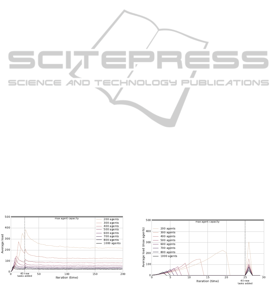
Figure 2: Scenario 1, 4000 tasks and an agent capacity of
500. The graph shows the impact of scheduling 40 new
tasks at iteration 25. For populations larger than 400 the
impact is minimal; all converge quickly.
ure 4 compares three separate runs of a simulation. To
ensure that these results are representative we also ran
parallel simulations with larger agent populations (up
to 1000), higher initial task load (up to 10,000) and for
up to 1000 iterations. A more detailed discussion of
these is outside the scope of this paper, the interested
reader is referred to (Hildmann and Martin, 2014) for
a more detailed discussion of the evaluation.
Note that we intentionally omit reporting the stan-
dard deviation because the randomly generated lo-
cations for tasks and agents (which do not change)
result in different lengths for the optimal schedules,
making the standard deviation meaningless unless re-
ported for much larger numbers of simulations.
Figure 2 illustrates how population size impacts
the convergence properties: besides the higher load
per agent for smaller populations, convergence to-
wards stable values is consistent across populations.
Figure 3 shows the average load of the max agents
for the same simulation as above. Note that a value
of zero indicates the absence of max agents, (i.e. all
tasks are allocated). Smaller populations take longer
to assimilate the initial task load into their schedules,
but the time it takes for the extra tasks seems to be
identical across population sizes.
The results in Figures 2 and 3 are for agent popu-
lations operating under comparatively low loads (i.e.
with a lot of excess capacity). We now briefly address
the question of how the approach performs when the
agents are approaching their maximum capacity.
Figure 4 shows the results of 3 separate runs. The
initial condition was 250 agents and 100 tasks, each
agent with a capacity of 75 and a visibility of 40. Ev-
ery 25 steps another 100 tasks are added to answer
the question whether the increasingly small (compar-
atively) additions or the decreasing remaining capac-
ity has a significant impact and to test the adaptivity
of the approach. From the graphs shown we can see
that even for high task loads the population quickly
reverts to the balancing stance and converge to an av-
Figure 3: As in Figure 2, showing the average loads of the
max agents (zero means there are no max agents). There is a
correlation between population size and iterations taken for
the initial task allocation; allocation of new tasks is uniform.
ICORES2015-InternationalConferenceonOperationsResearchandEnterpriseSystems
144
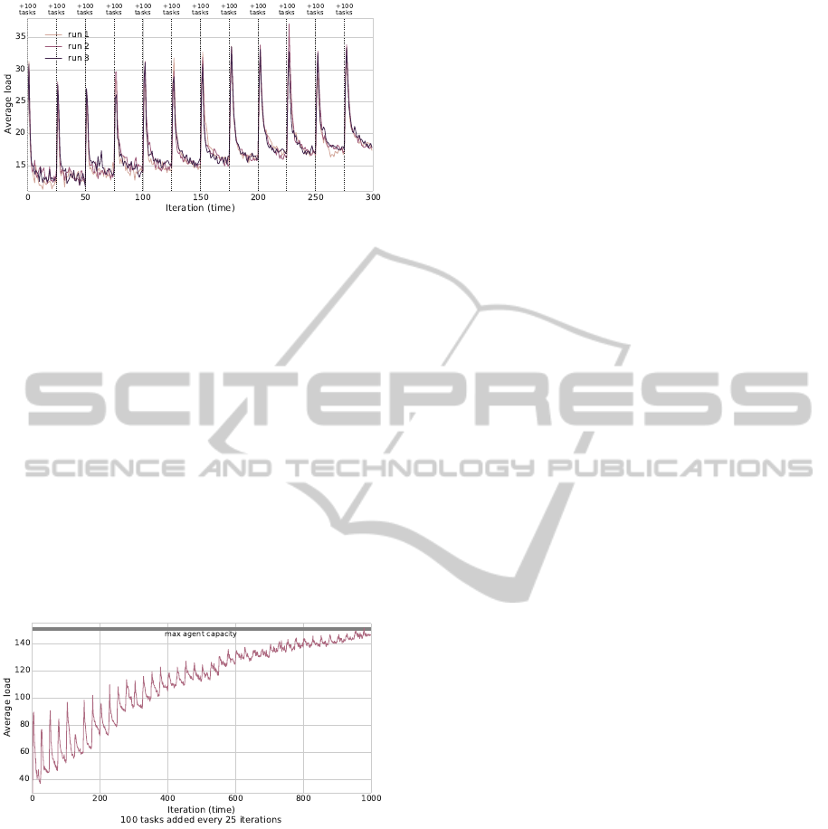
Figure 4: Scenario 2, 50 agents, capacity = 75. Every 25 it-
erations an additional 100 tasks are added, the graph shows
the average load of the agents from 3 separate runs. The
increase of the average is steadily increasing, as expected,
but the approach seems to continue to perform well.
erage which is consistently increasing in a linear way.
Figure 5 shows that even when approaching their
maximum capacity the performance of the population
does not deteriorate. It should be noted that in the
simulations the cost of a task is set to zero. If this
was not the case, there would be a linear increase in
the average load to match the aggregated cost of the
newly added tasks. The asymptotic curve seen above
results also from the fact that with increasing schedule
length the cost of adding a new task will (on average)
decrease (the more tasks you havethe higher the prob-
ability of two tasks being very close and thus having
a low distance cost associated with them).
Figure 5: Scenario 2 with 50 agents, capacity = 150, 100
tasks are added every 25 iterations: the graph shows the av-
erage load of the agents. Forlarge numbers of tasks (4000+)
the average load converges towards the agent’s capacity but
this does not affect the time to assimilate new tasks.
The above graphs support the claim that the
method does indeed scale and performs well. For a
detailed evaluation cf. (Hildmann and Martin, 2014).
5.3 Emergent Behaviour
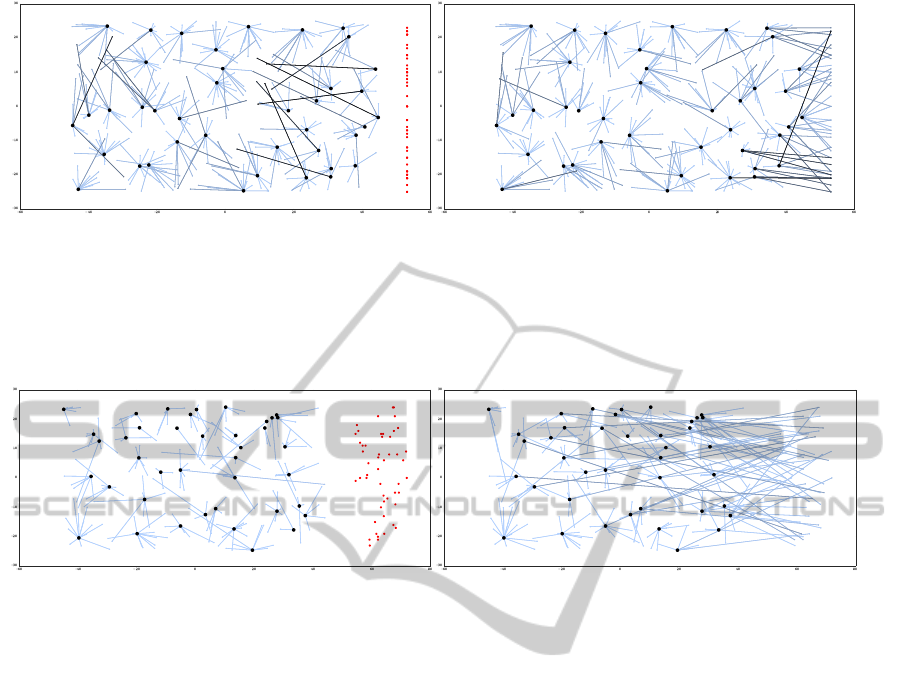
For the screenshots used to show the emergent be-
haviour we used scenarios 3 and 4. 50 agents were
placed randomly on the map, together with 500 ini-
tial tasks (which were supplemented by 50 additional
tasks at the outer edge of the map in iteration 50 (sce-
nario 3) or 60 (scenario 4). The range of the agents
was 350 and their visibility was set to 60.
We show two screenshots in Figure 6 that show the
simulation at the iteration when the new tasks are in-
troduced (a) as well as 40 iterations later when almost
all the tasks have been assimilated into the agents’
schedules. In comparison it is visible that the agents
on the left and in the middle of the map have taken on
a larger number of tasks to their respective right, i.e.
freeing agents on their right.
The screenshots in Figure 7 show the impact of
large visibility on the behaviour of the population.
Scenario 3 was used here. In addition, in this sim-
ulation the visibility was set equal to reachability, that
is, any task within reach was visible. Given that the
agents have quite some capacity left when the new
tasks are introduced this resulted in many agents as-
similating the new tasks. As a result, the average load
increased substantially, because the tasks were allo-
cated on a first come first serve basis with no regard
for its distance to the agent. While this was later miti-
gated when the agents had returned to balancing their
loads, the convergence to substantially longer.
6 DISCUSSION
We have presented an approach that, while not pro-
ducing efficient solutions with regard to the aggre-
gated workload, enable a population of agents to re-
act to changes in the environment and to dynamically
change according to changes in the problem space.
The graphs in the previous section show that the ap-
proach is scalable and that small as well as large prob-
lems can be handled.
Furthermore, the preliminary investigations (cf.
(Hildmann and Martin, 2014)) showed no dramatic
changes for growing problem space.
It was the stated aim of this paper to present the
mechanism that gives rise to the emergent behaviour
in the population. Through the two separate stances
the agents will, in effect, move tasks out of the realm
of the agents that can address the problem of unallo-
cated tasks. While the effect is rather hard to show on
still images, it is straight forward to see why this is
happening when one considers the 4 possible interac-
tions between agents: balanced agents will balance
the workload in the population of balanced agents.
Max agents will split into agents with very high load
and agents with very low load. The agents with a low
load will eventually assimilate the unallocated tasks,
while the agents with a high load are likely to lose
some of their load to balanced agents.
ResourceAllocationandSchedulingbasedonEmergentbehavioursinMulti-AgentScenarios
145
(a) (b)
Figure 6: The two screenshots, above, from a simulation running Scenario 4 with 400 initial tasks and 40 agents, each with a
maximum capacity of 220 and a visibility range of 65, illustrate the emerging behaviour of the population. In the map area,
each “star” is centered around a different agent’s depot, and the points connected to it radially represent the tasks the agent
currently has in its schedule. The darkness of the connection corresponds to its length. The red dots on the far right of the
map in (a) represent newly added and thus currently unscheduled tasks, all of which are scheduled in (b). When comparing
the right half of the maps in (a) and (b) we observe a shift in the orientation of the connections between tasks and agents.
Figure 7: The two pictures above illustrate the emergent behaviour in Scenario 3, using the same representation as Figure 6.
The settings are (in comparison to the above) half the initial tasks (200) for again 40 agents, which have a higher capacity
(320) and a much wider visibility (200). On a small map setting a high visibility range results in a large number of agents
assimilating the new tasks. This removes the collective behaviour where agents further from the tasks take on the load of
agents closer to the tasks. While this will allow for an quicker assimilation of all new tasks, it will take longer to distribute
the load fairly over the whole population. However, depending on the scenario, this might be a feasible parameter choice.
This should initially affect only balanced agents
that are close to max agents, but in time they will
share their load with other balanced agents, thereby
shedding some of their load to their colleagues as
well. As soon as the last unallocated task is assigned
to an agent all agents will become balanced and con-
tinuously strive to balance their loads.
We presented sufficient materials to allow the
reader a comparative implementation. The math pro-
vided is intentionally kept simple so as to facilitate the
implementation on standard computer hardware.
Restrictions to the Approach
The proposed method relies on a number of agents
working in proximity, such that the schedule assigned
to a specific agent can be partly absorbed into another
agent’s schedule. This is expected to require a critical
mass in order to outperform other approaches.
Furthermore, there is an upper limit to the degree
of change over time which the method can be ex-
pected to handle well. If the changes are too rapid
or dramatic, recalculating the entire solution might be
the better approach. This is due to the iterative nature
of the approach, which quickly adapts to changes and
“follows” moving centers of gravity in the problem
space. If such centers appear and disappear seemingly
at random it becomes impossible to follow them, and
thus the method will lose the edge over other ap-
proaches. However, we do not expect such dramatic
changes in the envisioned application areas.
One final issue should be raised here: we have
mentioned the Traveling Salesman Problem in the be-
ginning, and pointed out that it is known to be NP-
complete. We have then implemented our approach
and used a different way to calculate the cost of a
schedule. We haveinvestigated using the shortest path
from the depot through all tasks and back to the depot
as a cost function for a schedule, and will report on
these investigations separately; for now it suffices to
say that the computational cost of calculating the least
cost to address all tasks in a schedule is far outweigh-
ing the cost to calculate everything else implemented
for our approach. While this indicates that our ap-
ICORES2015-InternationalConferenceonOperationsResearchandEnterpriseSystems
146

proach can be implemented efficiently it also means
that for a real world application, the algorithm will
need to use some insight into the problem space to
decrease the computational cost associate with it. We
do consider this to be a relevant restriction.
It should be noted that the chosen problem is only
one example, used in this paper to illustrate the ap-
proach. By no means do we restrict the application
domain to service personnel; for example: the transi-
tion cost (distance) between tasks can be interpreted
as the overhead associated with the switching be-
tween tasks. Likewise, we use the term schedule, but
do not restrict the application of the presented method
nor the algorithm to schedules; e.g. the assignment
of resources to elements of non-ordered sets of tasks
(Beckers et al., 1994) can be addressed as well.
REFERENCES
Bartholdi, J. J. and Eisenstein, D. D. (1996). A produc-
tion line that balances itself. Operations Research,
44(1):21–34.
Beckers, R., Holland, O., and Deneubourg, J.-L. (1994).
From local actions to global tasks: stigmergy and col-
lective robots. In Proceedings of the Workshop on
Artificial Life, pages 181–189, Cambridge, MA. MIT
Press.
Bonabeau, E., Dorigo, M., and Theraulaz, G. (2000). Inspi-
ration for optimization from social insect behaviour.
Nature, 406:39–42.
Camazine, S., Deneubourg, J.-L., Franks, N. R., Sneyd,
J., Theraulaz, G., and Bonabeau, E. (2001). Self-
Organization in Biological Systems. Princeton Univ
Press.
Dussutour, A., Fourcassie, V., Helbing, D., and
Deneubourg, J.-L. (2004). Optimal traffic orga-
nization in ants under crowded conditions. Nature,
428:70–73.
Hassan, H. and Al-Hamadi, A. (2008). On compara-
tive evaluation of Thorndike’s psycho-learning exper-
imental work versus an optimal swarm intelligent sys-
tem. In Computational Intelligence for Modelling
Control Automation, 2008 International Conference
on, pages 1083 –1088.
Hildmann, H. and Martin, M. (2014). Adaptive scheduling
in dynamic environments. In 2014 Federated Confer-
ence on Computer Science and Information Systems
(FedCSIS), pages 1331–1336.
Holland, J. (1998). Emergence: From Chaos to Order. He-
lix books. Oxford University Press.
Luss, H. (2012). Equitable Resource Allocation: Models,
Algorithms and Applications. Information and Com-
munication Technology Series. Wiley.
Pinedo, M. (2012). Scheduling: Theory, Algorithms, and
Systems. SpringerLink : B¨ucher. Springer.
ResourceAllocationandSchedulingbasedonEmergentbehavioursinMulti-AgentScenarios
147
