
A Cooperative Game Approach to a Production Planning Problem
D. G. Ramírez-Ríos
1
, D. C. Landinez
2
, P. A. Consuegra
1
, J. L. García
1
and L. Quintana
1
1
Department of Industrial Engineering, Universidad de la Costa, Calle 58 # 55 - 66, Barranquilla, Colombia
2
Research Department, Fundación Centro de Investigación en Modelación Empresarial del Caribe,
Carrera 60 # 64 -122, Barranquilla, Colombia
Keywords: Cooperative Game Theory, Production Planning, Mixed Integer Linear Programming, Optimization,
Shapley Value.
Abstract: This paper deals with a production planning problem formulated as a Mixed Integer Linear Programming
(MILP) model that has a competition component, given that the manufacturers are willing to produce as
much products as they can in order to fulfil the market’s needs. This corresponds to a typical game theoretic
problem applied to the productive sector, where a global optimization problem involves production planning
in order to maximize the utilities for the different firms that manufacture the same type of products and
compete in the market. This problem has been approached as a cooperative game, which involves a possible
cooperation scheme among the manufacturers. The general problem was approached by Owen (1995) as the
“production game” and the core was considered. This paper identifies the cooperative game theoretic model
for the production planning MILP optimization problem and Shapley Value was chosen as the solution
approach. The results obtained indicate the importance of cooperating among competitors. Moreover, this
leads to economic strategies for small manufacturing companies that wish to survive in a competitive
environment.
1 INTRODUCTION
The high competition in the market has led many
companies to adopt supply chain management in
order to obtain better results and competitive
advantages to achieve a good positioning in them.
For this reason, businesses today search for an
optimal performance of their overall operations in
important areas like Production and Logistics
(Gimenez and Ventura, 2005). In order to do this,
many authors have provided contributions in this
field: Optimizing Inventory Operations (Hartman
and Dror, 2003); Optimal operations planning (Li et
al., 2003); Optimal price and return policy
(Mukhopadhyay and Setaputro, 2004); Optimal
operations of transportation fleet (Kang et al., 2008);
Optimal multi-stage logistic and inventory policies
(Hsiao, Lin & Huang, 2010); Optimal production
planning (Shi et al., 2011); Optimal deteriorating
items production inventory models (Widyadana and
Wee, 2011); Optimal production management
(Cadenillas et al., 2013); Optimal production
planning (Gong and Zhou, 2013); Optimal
transportation and business cycles (Das et al., 2014);
and Optimal dynamic policies for integrated
production (Chen, 2014).
Optimal production is directly related to
increased capacity and thus, a business is able to
offer more to their clients. Yet, the overall
performance of a business is not guaranteed by this,
given that there are many other factors (financial,
marketing, commercial) that affect the business’
performance and could be even more important than
production itself. Production planning optimization
problems have been approached to obtain the best
solution that maximizes or minimizes an objective
aimed by the business or group of businesses. This
solution, in many cases, seems an unrealistic
solution given that the businesses are observing a
static market. Getting a view of the competitors’
movements, on the other hand, makes the decision
even a more competitive one. Not only this, but if
integrating the competitor’s decisions in the market
to the production planning problem, could result in a
more plausible solution. When tackling this type of
problems, with a competition component involved, a
game theoretic solution approach should be
considered.
148
G. Ramírez-Ríos D., C. Landinez D., A. Consuegra P., L. García J. and Quintana L..
A Cooperative Game Approach to a Production Planning Problem.
DOI: 10.5220/0005220201480155
In Proceedings of the International Conference on Operations Research and Enterprise Systems (ICORES-2015), pages 148-155
ISBN: 978-989-758-075-8
Copyright
c
2015 SCITEPRESS (Science and Technology Publications, Lda.)

Production planning has been widely studied in
many of its components and applications in the
industry (Khaledi and Reisi-Nafchi, 2013), where
mathematical models have been the most
representative of this type of problems, on both
static and dynamic models (Missbauer and Uzsoy,
2011). Moreover, the competitive component of the
production planning has been approached by a few
authors and most of them have offered game
theoretic solutions to these problems. In (Zhou, Xiao
and Huang, 2010), the authors proposed a game
theoretic mathematical solution to generate the
optimal process plan for multiple jobs; (Manupati et
al., 2012) presented a scheme for generating optimal
process plans for multiple jobs in a networked based
manufacturing system by applying non-cooperative
games; (Aydinliyim and Vairaktarakis, 2013)
considered a competitive scheduling setting using a
cooperative game theoretic approach to achieve the
maximum savings possible.
Generally, production planning problems are
formulated using mixed integer linear programming
(MILP) models, issue that has had a great
development in the literature. Lütke Entrup et al.,
(2005) developed a MILP model that integrates
shelf-life issues into production planning and
scheduling. In (Ertugrul and Isik, 2009), the authors
presented a MILP model to wine production
planning. In (Doulabi et al., 2012), the formulation
of an open shop scheduling problem was developed
as two different MILP models. Jolayemi (2012)
developed a MILP model for scheduling projects
under penalty and reward arrangements, while in
(L'Heureux et al., 2013), the authors presented a
MILP model to solve a short term planning problem.
In (Mattik et al., 2014), an MILP optimization model
based on the block planning principle was developed
to obtain optimal production scheduling.
On the other hand, the application of game
theory to solve the production planning problem has
shown great impact during the last years. In (Li et
al., 2012), the authors developed an application of
game theory in planning and scheduling integration,
using Nash equilibrium to deal with multiple
objectives; In (Zamarripa et al., 2012), a multi-
objective MILP model was developed, to optimize
the planning of supply chain with a game theoretic
approach; In (Yin et al., 2013) a game theoretic
model to coordinate single manufacturer and
multiple suppliers with asymmetric quality
information was proposed.
Others have used cooperative game theory for
the formation of alliances in other contexts other
than production. For example, in (Okada, 2010) the
author proposed a cooperative game that describes
an economic situation in which n individuals can
communicate and form coalitions with each other
under the concept that such a strategic alliance
would increase individual income per participant.
The purpose of this paper is to illustrate an
approach to solving problems of production
planning with a competitive component through the
application of Game Theory.
2 PROBLEM FORMULATION
2.1 Mathematical Model for the
Production Planning Problem
We consider a production planning problem as a
MILP model in order to obtain the maximum
income for each of the manufacturers involved in
a specific market, which considers the production of
different products. The following model is
represented for each manufacturer.
Notation:
1,..., Product (good) type
1,…, Production facilities
1,…, Manufacturing firms
1,…, Type of raw materials
1,…, Client types
Parameters:
= Production capacities of product type at
production facility of the manufacturing firm.
= Raw material type available at
production facility of manufacturing firm.
= Quantity demanded of product type at
client.
= Price of product type offered to client by
manufacturing firml.
= Cost of manufacturing product type at
production facility by manufacturing firm.
= Quantity of raw material w required producing
product type
Variables:
Quantity of product type produced at
production facility by manufacturing firm sold to
client.
1,
0,
Objective Function:
ACooperativeGameApproachtoaProductionPlanningProblem
149

Maximize
(1)
Subject to
∀,
,
(2)
,
∀,
,
(3)
,
∀,
(4)
∈
∀,
,,
(5)
Equation (1) establishes the objective function of the
production problem, which aims to maximize the
total utilities of the manufacturers. Equation (2), (3)
and (4) establish capacity and demand restrictions.
For a single manufacturing firm this model is
simple (the decision variable
should not be
included) and an optimal solution is guaranteed,
which makes the capacity restriction the main
concern to obtaining greater income for each
manufacturer.
Given that there are multiple manufacturers
integrated in the same optimization problem, when
competing in the same market, the solution is not
that simple. Moreover, if some of the manufacturing
companies are small and, as an overall, the industry
is affected by external competitors that are
threatening to take away a part of their own market,
a strategy besides working at optimal conditions, has
to be implemented by the manufacturers.
2.2 Cooperative Game Model
The "Production Game” (Owen, 1995) is defined as
a set of players
1,2,…,
, each player has a
batch of kinds of raw material. Player 1 has
units of raw material 1,
units of raw material 2,
and
,
units of raw material ; Player 2 has
units
raw material 1,
units of raw material 2
and
,
units of raw material ; player 3 has
units of raw material 1,
units of raw material 2,
and
,
units of raw material ,…, player has
units of raw material 1,
units of raw
material 2,…,
,
units of raw material . The
products do not have value for themselves, except
that they are used to produce goods
,
,…,
which can be sold at prices set in the market. A
linear production process is assumed, in which one
unit of the product 1 requires
raw material 1,
units of the raw material 2 and
,
units of the
raw material ; a unit of the product 2 requires
units of raw material 1,
units of raw material
units 2 and
,
units of the raw material , one
unit of the product requires
units of raw
material 1,
units raw material 2 and
,
units
of the raw material . Products
,
,…,
can be
sold at
,
,…,
dollars respectively.
When a coalition is formed, members will
contribute to each of their products in order to
maximize profits from the sale of products on the
market. Therefore, the characteristic function is
given by the following linear equation:
v
S
(6)
Subject to:
,∀
(7)
Where:
∈
(8)
3 SOLUTION APPROACH
3.1 Application of the MILP to the
Cooperative Game Model
The model described in section 2.1 is integrated to
the Cooperative Game Model described in section
2.2. For the implementation of the game, the
following cooperation strategies were considered:
When cooperating, each player is allowed to
share its capacity with the others that form the
coalition.
Utilities are transferable among players that form
the same coalition.
3.1.1 Definition of the Cooperative Game
Consider the manufacturers, players of the game.
Each player has a manufacturing facility with
available raw materials for production and clients
requiring each type of product. Each one yields for
the maximum payoff, according to the MILP
formulated in section 2.1. When cooperating, the
production is set on two strategies: (i) more capacity
ICORES2015-InternationalConferenceonOperationsResearchandEnterpriseSystems
150

is available and (ii) prices are stabilized according to
the market’s needs.
3.1.2 Characteristic Function
Given the optimal income function presented
previously and for the general problem, the
resulting characteristic function evaluated is:
v
S
∗
∈
(9)
where,
∗
is the average price of product type
offered to client for all players belonging to the
coalition , That is, every player belonging to the
coalition , offers to each client , a product type
with a
∗
price. On the other hand, the cost involved
corresponds to the facility that is actually managing
the production of the type of product sold. The
facilities chosen to manufacture a product are
subject to the capacity restriction that was previously
stated in the MILP formulation, and adapted to the
cooperative model as follows in eq. 10.
∀,
,
(10)
3.2 Shapley Value
Shapley Value is a solution approach to cooperative
games and is given by the following equation:
φ
1
!
1
!
!
⊂
(11)
Where is any finite company, with
|
|
.
This formulation expresses the Shapley value for
each player in a game as a weighted sum of
terms of the form
, which is the
contribution of player to coalition (Roth, 1988).
In this way, the contribution of each player can
be calculated by using an algorithm that evaluates
the Shapley Value, which is explained in the
following sections.
3.2.1 Solution Algorithm
Calculating the Shapley Value has been a research
topic of interest. Its computational complexity is
combinatorial given that it requires knowing all
possible combinations among the different
players, that is, 2
1. The model proposed in this
paper presents an efficient algorithm that can be
applied to many players, given that it integrates the
probabilistic aspect of the Shapley Value formula
and the possible margin of contribution that any
player is able to make in a coalition. Similar to the
expected value a decision making model under
uncertainty restrictions, the Shapley Value is the
expected value of each player under the different
coalition scenarios. The table 1 explains the
calculations executed in this algorithm with an
example of four players.
Table 1: Shapley Value calculation for 4 players.
th pl.
1 2 3 4
1 v(1)
v(1,2) – v
(2) + v (1,3)
– v(3) + v
(1,4) - v (4)
v(1,2,3) -
v (2.3) +
v(1,2,4) -
v(2.4) +
v(1,3,4) -
v(3,4)
v
(1,2,3,4)
-
v(2,3,4)
2 v(2)
v (1,2) - v
(1) + v (2,3)
- v (3) + v
(2,4) - v (4)
v (1,2,3) -
v (1,3) + v
(1,2,4) - v
(1,4) + v
(2,3,4) - v
(3,4)
v
(1,2,3,4)
-v
(1,3,4)
3 v(3)
v (1,3) - v
(1) + v (2,3)
- v (2) + v
(3,4) - v (4)
v (1,2,3),
v (1,2) + v
(2,3,4), v
(2,4) + v
(1,3,4), v
(1,4)
v
(1,2,3,4)
-v
(1,2,4)
4 v(4)
v (1,4) -
v (1) + v
(2,4) - v (2)
+ v (3,4), v
(3)
v (1,2,4),
v (1,2) + v
(1,3,4), v
(1,3) + v
(2,3,4), v
(2,3)
v
(1,2,3,4)
-v
(1,2,3)
3.2.2 Pseudo Code
The resulting program code for the solution
algorithm generated is showed in the Appendix
section.
This solution approach was first applied to other
applications related to supply chain, resulting in
interesting results. In the electric energy industry,
where a two-level game was proposed, in which the
first one looks for a Stackelberg Equilibrium
solution where the leader is a generator, in
particular, then the second-level obtains the
coordination among a group of marketers following
a cooperative game, where Shapley Value is
calculated for each player as a result of their
coordination (Guzmán et al., 2008). Also, in the
furniture industry, with respect to the competitive
value of both supplier and manufacturing companies
(Puello-Pereira and Ramírez-Ríos, 2014).
ACooperativeGameApproachtoaProductionPlanningProblem
151
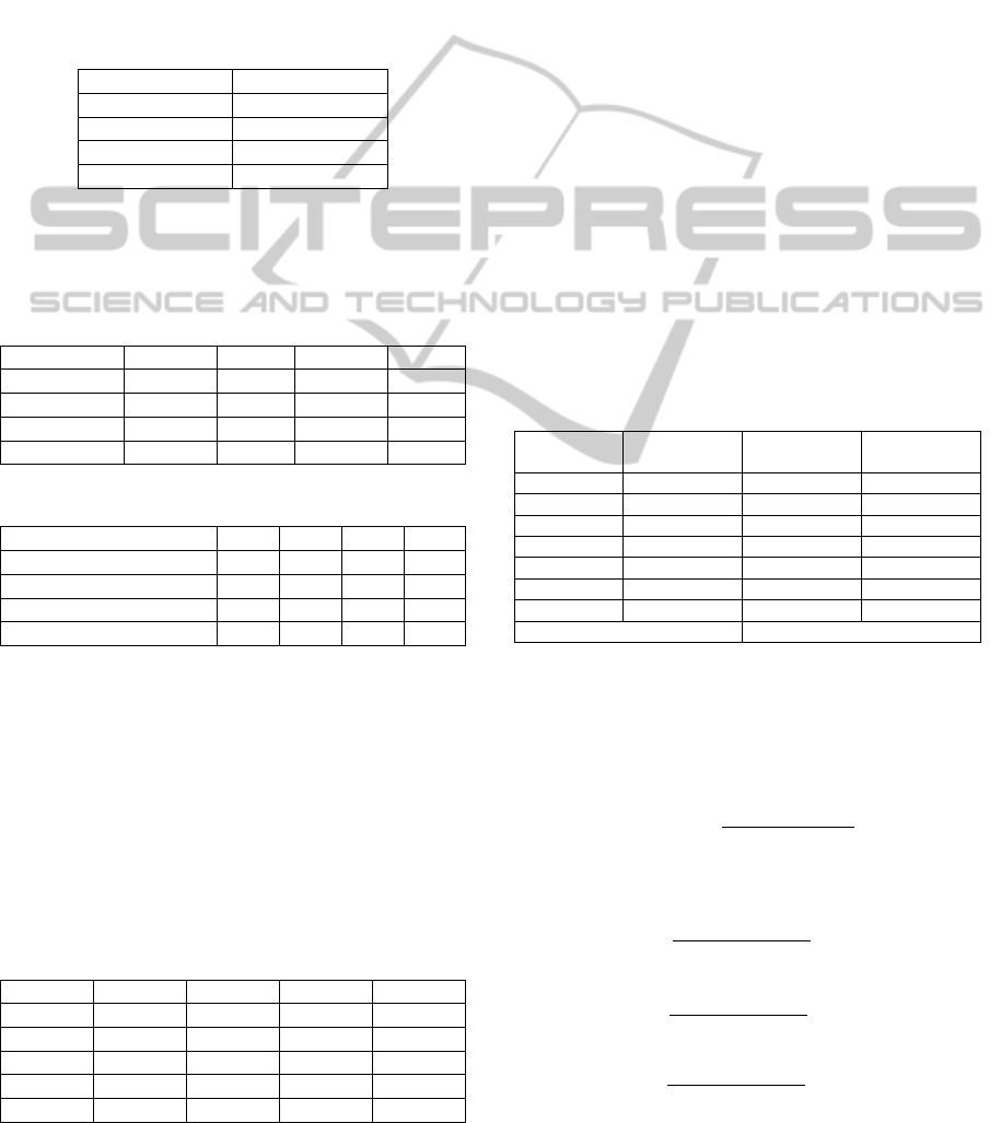
4 RESULTS
4.1 Numerical Example
For the numerical example, a 4-player game is
considered, where each player represents a
manufacturing company that competes for a single
client with four different products. The information
below includes the market price and consumption of
raw material per type of product.
Table 2: Market price:
Product type
Price
1 40
2 50
3 45
4 35
It is assumed that the fabrication of product
requires four different materials in the proportions
showed in Table 4.
Table 3: Amount of raw material.
Raw material Player 1 Player 2 Player 3 Player 4
1 200 150 130 180
2 100 210 190 140
3 50 155 230 160
4 300 135 180 90
Table 4: Raw material requirement.
Row material
1 5 6 6 5
2 6 2 1 5
3 1 2 5 1
4 3 5 1 6
4.1.1 Optimal Solution for the Competitive
Model
This problem was solved initially as global
optimization model that didn’t consider possible
cooperation among the agents.
By using an optimization engine (GAMS), an
optimal solution was generated, with a total utility of
$5.155, where the optimal value, corresponding to
each player, is presented in table 5.
Table 5: Solution generated.
P. type Player 1 Player 2 Player 3 Player 4
Prod 1 10 0 2 0
Prod 2 20 25 20 15
Prod 3 0 0 0 15
Prod 4 0 0 0 0
Utilities 1400 1250 1080 1425
4.1.2 Cooperative Game Solution to the
Problem
For this numerical example, the possible coalitions
are the following:
1, 2, 3, 4, 1,2,
1,3, 1,4, 2,3, 2,4, 3,4, 1,2,3,
1,2,4, 1,3,4, 2,3,4 y, 1,2,3,4.
According to the solution approach implemented,
after weighing the coalitions, an optimization engine
is integrated to generate the optimal value for each
scenario, resulting in each contribution to the
coalition, as was presented in table 1.
For each scenario generated, the FO value for
each player is considered as the contribution of each
one to the coalition. In the first case, when
considering individual coalitions, that is, {1}, {2},
{3} and {4}, the optimal solution would be the ones
considered in the optimization model previously
solved if solved individually. Thus for Player 1, it
turns to be optimal to manufacture 10 units of
product 1 and 20 units for product 2. Nevertheless,
when it comes to sharing demanded quantity, the
solutions change for the other players.
After solving for all scenarios, optimal values for
each coalition are given in the following table.
Table 6: Optimal value.
Coalition
Optimal
value
Coalition
Optimal
value
v (1) 1400 v (2,3) 2333.3
v (2) 1250 v (2,4) 2687.5
v (3) 1083.33 v (3,4) 2583.3
v (4) 1425 v (1,2,3) 4000
v (1,2) 2916.66 v (1,2,4) 4416.66
v (1,3) 2750 v (1,3,4) 4250
v (1,4) 3166.66 v (2,3,4) 3833.33
v (1,2,3,4) 5500
4.1.3 Shapley Solution
In the previous subsection coalitions were formed
and also optimal values for each coalition were
calculated, the next step is find optimal coalitions
s1
!
ns
!
n!
:
(12)
We replace for each player:
11!41!
4!
0,25
:
(13)
21!42!
4!
0,083
:
(14)
31!4 3!
4!
0,083
:
(15)
ICORES2015-InternationalConferenceonOperationsResearchandEnterpriseSystems
152
41!44!
4!
0,25
:
(16)
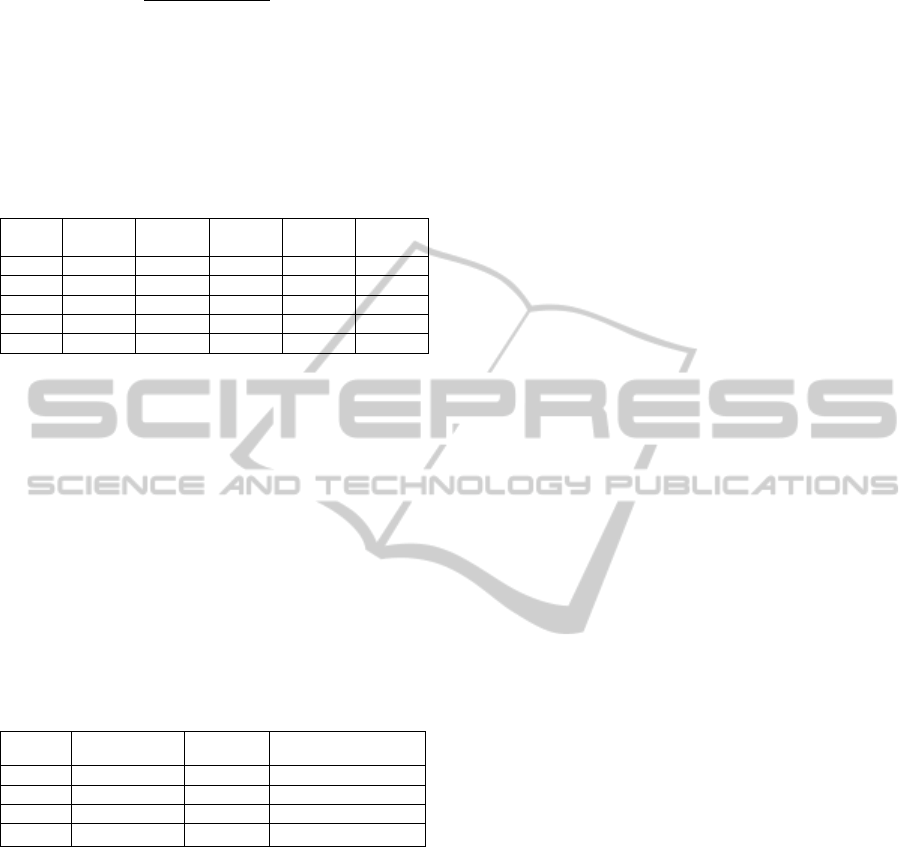
The resulting solution that gives the Shapley Value
is given in table 7, as shown in the last column,
which is considered as the payoff that should be
assigned to each player in the coalition
1,2,3,4
, also known as the grand coalition.
Table 7: Shapley values.
th
player
1 2 3 4 ᶲ
1 1400 5075 5062.5 1667 1611.5
2 1250 4029 3750 1250 1273
3 1083 3592 3312.5 1083 1117
4 1425 4500 4500 1500 1498
0.25 0.0833 0.0833 0.25 5500
According to the Shapley value, the distribution
of the profits associated with each player in the
grand coalition are as follows:
For player one USD $ 1,611.45.
For player two USD $ 1,273.26.
For the player three USD $ 1,273.26.
For the player four USD $ 1,273.26.
Value of grand coalition USD $ 5,500.00.
The results, as compared to the individual payoffs
observed in table 5, show the feasibility of the
solution and the economic incentive for cooperating.
Table 8 show the comparison of the results obtained.
Table 8: Results compared.
Player Individual SV % Improvement
1 1400 1611,5 15%
2 1250 1273 2%
3 1083 1117 3%
4 1425 1498 5%
4.2 Analysis Results Generated
After solving the numerical example shown above, it
can be observed that cooperation is possible among
competitors, which assume the share of demanded
quantities for each one of the products offered. The
grand coalition sets an overall of $5.500, much
greater than what the global model considered
initially, $5.155. In the resulting cooperative model,
player 1 is most strategically benefited as shown by
the Shapley values generated. Yet, overall, all
players are benefitted, obtaining greater benefits
than operating individually.
5 CONCLUSIONS
The increase of market competitiveness generates a
growing interest in companies to improve their
processes and operations in order to obtain
satisfactory results and become well positioned. This
has encouraged many of them to integrate with their
competitors where the implementation of strategies
focused on collaboration between several companies
with a common goal. Nevertheless, this is not
always true due to the lack of incentives that
businesses have to cooperate. For this reason, many
companies decide to continue working
independently. In this particular case, cooperative
game theory offers solutions such as the Shapley
Value that allows an efficient distribution of
incentives among each player, thus, resulting in a
contribution received by each player, according to
its objective function.
In this paper, we considered a problem of
production planning in manufacturing companies,
with a cooperative game model that integrated with
MILP models that made possible the determination
of optimal coalitions and the amount of each type of
product to be manufactured by each player. The
results generated, indicate that involving
competition to obtain optimal benefits is not as
simple as solving for a MILP model. Involving
competition requires generating previous decisions,
which are considered in several scenarios that must
be evaluated. Moreover, if cooperation is
considered, the implications make it a more dynamic
and complex model.
The Shapley value calculation determine an
efficient way of distributing their income and a
solution algorithm was implemented in order to
calculate the value among many companies.
This solution approach demonstrated that
cooperation is not only recommended at a strategic
level, but also is considered an important strategy for
companies that are struggling in a competitive
market and are striving to succeed.
Future research directions are considered
reducing the complexity of coalition formation when
addressing Shapley Value. Also, there are multiple
applications where cooperation is needed and more
and more companies are searching for a way to
cooperate without losing money.
ACKNOWLEDGEMENTS
This research is supported by Universidad de la
Costa (CUC) and Fundación Centro de Investigación
ACooperativeGameApproachtoaProductionPlanningProblem
153

en Modelación Empresarial del Caribe (FCIMEC).
This paper responds to the project “Cooperative
Game Theory and Shapley Value” that integrates the
research groups SimOpt and Producom.
REFERENCES
Aydinliyim, T., Vairaktarakis, G. L., 2013. A cooperative
savings game approach to a time sensitive capacity
allocation and scheduling problem. Decision Sciences,
44(2), 357-376.
Cadenillas, A., Lakner, P., Pinedo, M., 2013. Optimal
production management when demand depends on the
business cycle. Operations Research, 61(4), 1046-
1062.
Chen, L. T., 2014. Optimal dynamic policies for integrated
production and marketing planning in business-to-
business marketplaces. International Journal of
Production Economics, 153, 46-53.
Das, B. C., Das, B., Mondal, S. K., 2014. Optimal
transportation and business cycles in an integrated
production-inventory model with a discrete credit
period. Transportation Research Part E: Logistics and
Transportation Review, 68, 1-13.
Doulabi, S. H. H., Avazbeigi, M., Arab, S., Davoudpour,
H., 2012. An effective hybrid simulated annealing and
two mixed integer linear formulations for just-in-time
open shop scheduling problem. The International
Journal of Advanced Manufacturing Technology,
59(9-12), 1143-1155.
Ertugrul, I., Isik, A. T., 2009. Production Planning for a
Winery With Mixed Integer Programming Model. Ege
Academic Review, 9(2), 375-387.
Gimenez, C., Ventura, E., 2005. Logistics-production,
logistics-marketing and external integration: their
impact on performance. International journal of
operations & Production Management, 25(1), 20-38.
Gong, X., Zhou, S. X., 2013. Optimal production planning
with emissions trading. Operations Research, 61(4),
908-924.
Guzman, L., Ramírez Ríos, D. G., Yie, R., Ucros, M.,
Acero, K., Paternina, C. D., 2008. Modelos de
planificación cooperativa de recursos energéticos.
Ediciones Uninorte, Barranquilla, 178p.
Hartman, B. C., Dror, M., 2003. Optimizing centralized
inventory operations in a cooperative game theory
setting. IIE Transactions, 35(3), 243-257.
Hsiao, Y. C., Lin, Y., Huang, Y. K., 2010. Optimal multi-
stage logistic and inventory policies with production
bottleneck in a serial supply chain. International
Journal of Production Economics, 124(2), 408-413.
Jolayemi, J. K., 2012. Scheduling of projects under
penalty and reward arrangements: a mixed integer
programming model and its variants. Academy of
Information & Management Sciences Journal, 15(2).
Kang, S., Medina, J. C., Ouyang, Y., 2008. Optimal
operations of transportation fleet for unloading
activities at container ports. Transportation Research
Part B: Methodological, 42(10), 970-984.
Khaledi, H., Reisi-Nafchi, M., 2013. Dynamic production
planning model: a dynamic programming approach.
The International Journal of Advanced Manufacturing
Technology, 67(5-8), 1675-1681.
L'Heureux, G., Gamache, M., Soumis, F., 2013. Mixed
integer programming model for short term planning in
open-pit mines.
Mining Technology, 122(2), 101-109.
Li, P., Wendt, M., Wozny, G., 2003. Optimal operations
planning under uncertainty by using probabilistic
programming. Foundations of Computer-Aided
Process Operations (FOCAPO 2003), Coral Springs,
FL.
Li, X., Gao, L., & Li, W., 2012. Application of game
theory based hybrid algorithm for multi-objective
integrated process planning and scheduling. Expert
Systems with Applications, 39(1), 288-297.
Lütke Entrup, M., Günther, H. O., Van Beek, P., Grunow,
M., & Seiler, T., 2005). Mixed-Integer Linear
Programming approaches to shelf-life-integrated
planning and scheduling in yoghurt production.
International Journal of Production Research, 43(23),
5071-5100.
Manupati, V. K., Deo, S., Cheikhrouhou, N., Tiwari, M.
K., 2012. Optimal process plan selection in networked
based manufacturing using game-theoretic approach.
International Journal of Production Research, 50(18),
5239-5258.
Mattik, I., Amorim, P., Günther, H. O., 2014. Hierarchical
scheduling of continuous casters and hot strip mills in
the steel industry: a block planning application.
International Journal of Production Research, 52(9),
2576-2591.
Missbauer, H., Uzsoy, R., 2011. Optimization models of
production planning problems. In Planning
Production and Inventories in the Extended Enterprise
(pp. 437-507). Springer US.
Mukhopadhyay, S. K., Setoputro, R., 2004. Reverse
logistics in e-business: optimal price and return policy.
International Journal of Physical Distribution &
Logistics Management, 34(1), 70-89.
Okada, A. The Nash bargaining solution in general n-
person cooperative games. Journal of Economic
Theory 2010, Vol. 145, pp 2356-2379.
Owen, G., 1995, Game Theory. In San Diego: Academic
Press. 447p.
Puello Pereira, N. & Ramírez Ríos, D.G., 2014. Un
modelo de juegos cooperativos aplicado a cadenas de
suministro para maximizar la competitividad de los
clusters. In Revista Ingeniare, Paper submitted for
publication.
Roth, A., 1988. The Shapley Value. In Cambridge
University Press, 1988. ISBN 0-521-36177-X.
Shi, J., Zhang, G., Sha, J., 2011. Optimal production
planning for a multi-product closed loop system with
uncertain demand and return. Computers &
Operations Research, 38(3), 641-650.
Widyadana, G. A., Wee, H. M., 2011. Optimal
deteriorating items production inventory models with
random machine breakdown and stochastic repair
ICORES2015-InternationalConferenceonOperationsResearchandEnterpriseSystems
154

time. Applied Mathematical Modelling, 35(7), 3495-
3508.
Yin, S., Nishi, T., & Zhang, G., 2013. A Game Theoretic
Model to Manufacturing Planning with Single
Manufacturer and Multiple Suppliers with
Asymmetric Quality Information. Procedia CIRP, 7,
115-120.
Zamarripa, M., Aguirre, A., & Méndez, C., 2012.
Integration of Mathematical Programming and Game
Theory for Supply Chaina Planning Optimization in
Multi-objective competitive scenarios. Computer
Aided Chemical Engineering,30, 402-406.
Zhou, G., Xiao, Z., Jiang, P., & Huang, G. Q., 2010. A
game-theoretic approach to generating optimal process
plans of multiple jobs in networked manufacturing.
International Journal of Computer Integrated
Manufacturing, 23(12), 1118-1132.
APPENDIX
Solution algorithm
Count = number of coalitions formed.
Count < 2
m
-1
begin
g = m, w= 0
For l = 1 to m
S
lg
= assign l to coalition S
v(S
lg
)=Max f(x)
Next l
w= w + m
Do while w <= Count
Do
z=1
h=g-1
For j = 1 to h
Do
S
wh
= j
For i = h+1 to g
S
wi
= j+z
v(S
wi
)= Max f(x
j
) jS
wi
z = z +1
Next i
w=w+1
while j+z = m
Next j
h= h-1
while h > 0
Loop
For l=1 to m
For r=1 to g
Calculate marginal payoffs
MV
r
= sum
r
[v(S
rl
)-v(S
rl
-l)]
Calculate p
r
Next r
Next l
Calculate shapley value SV
l
SV
l
=sum
l
[p
r
*MV
l
]
end
ACooperativeGameApproachtoaProductionPlanningProblem
155
