
Normalised Diffusion Cosine Similarity and Its Use
for Image Segmentation
Jan Gaura and Eduard Sojka
V
ˇ
SB - Technical University of Ostrava, Faculty of Electrical Engineering and Computer Science,
17. listopadu 15, 708 33 Ostrava-Poruba, Czech Republic
Keywords:
Diffusion Distance, Cosine Similarity, Image Segmentation.
Abstract:
In many image-segmentation algorithms, measuring the distances is a key problem since the distance is often
used to decide whether two image points belong to a single or, respectively, to two different image segments.
The usual Euclidean distance need not be the best choice. Measuring the distances along the surface that is
defined by the image function seems to be more relevant in more complicated images. Geodesic distance, i.e.
the shortest path in the corresponding graph, or the k shortest paths can be regarded as the simplest methods.
It might seem that the diffusion distance should provide the properties that are better since all the paths (not
only their limited number) are taken into account. In this paper, we firstly show that the diffusion distance
has the properties that make it difficult to use it image segmentation, which extends the recent observations of
some other authors. Afterwards, we propose a new measure called normalised diffusion cosine similarity that
is more suitable. We present the corresponding theory as well as the experimental results.
1 INTRODUCTION
Measuring the distance is an important problem in
clustering and image segmentation. The distance is
used as a quantity that makes it possible to decide
whether two image pixels belong to one or two dif-
ferent clusters (image segments). The Euclidean dis-
tance (i.e. the direct straight-line distance) need not
be the best choice. In images, the image points form a
certain surface in some space. Measuring the distance
along this surface promises better results.
The geodesic distance (Papadimitriou, 1985;
Surazhsky et al., 2005) measures the length of the
shortest path lying entirely on the surface. The prob-
lem is that the geodesic distance can be influenced
significantly by relatively small disturbances in image
since only one (and ”thin”) path on the surface deter-
mines the distance. In (Eppstein, 1998), the possibil-
ity of computing k shortest paths is discussed. This
can be viewed as an attempt to take into considera-
tion the connection that is not thin, but has a certain
width, which reduces the influence of disturbances
and noise.
The resistance distance is a metric on graphs
(Klein and Randi
´
c, 1993; Babi
´
c et al., 2002). The
resistance distance between two vertices of graph is
equal to the effective resistance between the corre-
sponding nodes in an equivalent electrical network
(regular grid in this case). The resistances of edges in
the network increase with the increasing local image
contrast. Intuitively, the resistance distance explores
all the existing paths between two points whereas the
geodesic distance explores only the shortest of them.
It was shown that the resistance distance is equiv-
alent to so called commute-time distance (Fouss et al.,
2007; Yen et al., 2007; Qiu and Hancock, 2007)
which is the distance based on summing the diffu-
sion distance in time. Diffusion is a process during
which a certain substance, e.g. heat or electric charge
diffuses from the places of its greater concentration
to the places where the concentration is lower. The
mathematical description can be built on the diffu-
sion equation (i.e. can be physically based) or on the
Markov matrices describing the random walker tech-
nique (Grady, 2006). The diffusion maps were sys-
tematically introduced in (Nadler et al., 2005; Coif-
man and Lafon, 2006). Although further papers ap-
pear, e.g. (Lipman et al., 2010), almost nothing is re-
ported about successful use of diffusion distance for
image segmentation. This can be regarded as surpris-
ing since, at a first glance, the method should have the
properties that are useful. For measuring every dis-
tance, it examines many paths on the image surface.
In this paper, we show that the diffusion distance
121
Gaura J. and Sojka E..
Normalised Diffusion Cosine Similarity and Its Use for Image Segmentation.
DOI: 10.5220/0005220601210129
In Proceedings of the International Conference on Pattern Recognition Applications and Methods (ICPRAM-2015), pages 121-129
ISBN: 978-989-758-076-5
Copyright
c
2015 SCITEPRESS (Science and Technology Publications, Lda.)

need not be beneficial for measuring distances in im-
age segmentation. The reason is that the influence
of different sizes of image segments may overshadow
the influence of the edges between them (i.e. the dif-
ferences in brightness or colour). This finding extends
the observations of some other authors that appeared
recently (von Luxburg et al., 2014). We introduce a
new measure called normalised diffusion cosine simi-
larity in which the mentioned problem is significantly
reduced. The computational technique (as well as the
time complexity) remains similar as is usually pre-
sented for the diffusion distance, i.e. it is based on
the spectral decomposition of the Laplacian matrix.
The paper is organised as follows. In the following
section, we recall the needed theoretical background.
In Section 3, the problems of diffusion distance are
explained. The new similarity is introduced in Section
4. Section 5 is devoted to the experimental results.
The concluding remarks are given in Section 6.
2 DIFFUSION DISTANCE AND
CLUSTERING
The diffusion-based methods are usually formulated
by making use of the diffusion equation
∂ f (t,x)
∂t
= div(g( f (t,x), x)∇ f (t,x)) , (1)
where f (t,x) is a potential function (e.g. concentra-
tion, temperature, charge) evolving in time; g(·) is a
diffusion coefficient (generally, it is a function). In
some applications, the coefficient does not depend on
f (t, x). If g(·) reduces to a constant G, the right-hand
side of Eq. (1) reduces to G∇
2
f (t, x). In our con-
text, f (t,x) has the meaning of evolving image bright-
ness or colour. The process of evolving starts at t = 0;
f (0, x) is a given input image.
In the discrete case, the problem is formulated in a
graph (Sharma et al., 2011). The diffusion properties
are represented by edge weights that can be under-
stood as proximity between the neighbouring nodes
connected by the corresponding edge. The weights
may again be considered evolving in time or constant.
In this paper, we follow the latter option. The diffu-
sion equation can now be written in the form of
∂
~
f (t)
∂t
= L
~
f (t), (2)
where L is the Laplacian matrix containing the
weights of edges;
~
f (t) is a vector whose entries cor-
respond to the potential in the particular graph nodes,
i.e.
~
f (t) = ( f
1
(t),.. ., f
n
(t))
>
(we suppose the graph
with n nodes). The weight, denoted by w
i, j
, of the
edge connecting the nodes i and j is often considered
according to the formula
w
i, j
= e
−
kc
i, j
k
2
2σ
2
, (3)
where c
i, j
denotes the grey-scale or colour contrast
between the nodes.
The solution of Eq. (2) can be found in the form
of (Sharma et al., 2011)
~
f (t) = H(t)
~
f (0) , (4)
where H(t) is a diffusion matrix. The entry h
t
(p,q) of
H(t) expresses the amount of a substance that is trans-
ported from the q-th node into the p-th node (or vice
versa since h
t
(p,q) = h
t
(q, p)) during the time inter-
val [0,t]. It can be shown that the following formula
for H(t) ensures that Eq. (2) is satisfied
H(t) =
n
∑
k=1
e
−λ
k
t
~u
k
~u
>
k
, (5)
where λ
k
and~u
k
, respectively, stand for the k-th eigen-
value and the k-th eigenvector of L. Let u
i,k
be the i-th
entry of the k-th eigenvector. For each graph vertex,
the vector of new coordinates can be introduced
~x
i
(t) =
e
−λ
1
t
u
i,1
,e
−λ
2
t
u
i,2
,. . . ,e
−λ
n
t
u
i,n
. (6)
If the coordinates are assigned in this way, we call it
diffusion map (Coifman and Lafon, 2006; Lafon and
Lee, 2006). This vector can be used for clustering the
vertices, which will be discussed later. By making use
of this vector, the entries of the diffusion matrix can
be expressed as the following dot product
h
2t
(p,q) = h~x
p
(t),~x
q
(t)i. (7)
The square of diffusion distance is defined as a
sum of the squared differences of the concentrations
caused by putting the unit concentration into the p-
th node and into the q-th node, respectively, which
corresponds to the formula
d
2
t
(p,q) =
n
∑
i=1
[h
t
(i, p) −h
t
(i,q)]
2
. (8)
After some effort, the following formula can be
deduced from Eq. (8)
d
2
t
(p,q) = h
2t
(p, p) −2h
2t
(p,q) + h
2t
(q,q)
= k~x
p
(t) −~x
q
(t)k
2
, (9)
which shows that introducing the coordinates accord-
ing to Eq. (6) may be seen as creating a diffusion map,
which is a map created in a similar sense as in (Tenen-
baum et al., 2000), where the idea was presented that
measuring the distance along the data manifold in
ICPRAM2015-InternationalConferenceonPatternRecognitionApplicationsandMethods
122
some space can be done by transforming the prob-
lem into a new space in such a way that the Euclidean
distance in the new space is equal to the distance mea-
sured on the data manifold in the original space.
Diffusion clustering is based on the idea to use the
coordinates introduced in Eq. (6) for clustering the
graph nodes, i.e. the image pixels (Nadler et al., 2005;
Lafon and Lee, 2006; Huang et al., 2011). The time
t can be used to set the level of details that is desired.
Often, the k-means clustering method is mentioned
in this context (Lafon and Lee, 2006; Huang et al.,
2011). It is believed that much less than n coordinates
are needed in practice.
3 THE PROBLEMS OF
DIFFUSION DISTANCE
In this section, we show that the diffusion distance
has the properties that make it difficult to use it for
image segmentation. We show that the value of diffu-
sion distance between two image points does not nec-
essarily give a good clue whether or not they belong
to one image segment. We note that a certain criti-
cism in a similar sense has already been published for
the commute-time distance. In (von Luxburg et al.,
2014), the authors came to the conclusion that the
commute-time distance in graph does not reflect its
structure correctly if the graph is large. We continue
in this direction and show some further problems that
are relevant for image segmentation. We also show
that the problems appear not only for the commute-
time (resistance) distance, but also for the diffusion
distance, i.e. they cannot be avoided by a certain suit-
able choice of time.
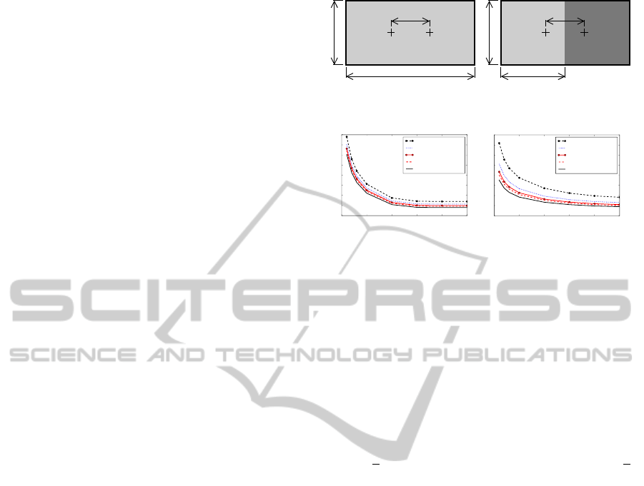
Consider two points, denoted by p, q, in image.
We study two situations (Fig. 1): (i) Both the points
are placed in an image containing one rectangular
area with a constant brightness; the size of image is
w ×h pixels. (ii) The size of image is w ×h pixels
again, but the image area is now split by the vertical
line into two halves (areas); the brightness is constant
inside each area; the difference of brightness between
the areas is equal to 1; each of the points is placed
in one area. The Euclidean distance between p and q
measured in the xy plane is denoted by a (Fig. 1). We
traditionally call these situations as ”without edge”
and ”with edge”, respectively. Clearly, from the point
of view of image segmentation, these two situations
are substantially different. In the second case, we ex-
pect two image segments and a big distance between
p and q. In the first case, only one image segment and
a small distance between p and q are expected.
A simple theoretical consideration might be useful
p
q
h
w
a
p
q
w/2
a
h
Figure 1: Two points (p,q) placed into an image containing
a single area (left image) or two areas (right image).
30x11 30x21 30x31 30x41 30x51
Area Size [px]
0.04
0.06
0.08
0.10
0.12
0.14
0.16
0.18
0.20
Diffusion Distance, t= 25
With Edge σ=0.4
With Edge σ=0.5
With Edge σ=0.6
With Edge σ=0.7
Without Edge σ=0.5
30x11 30x21 30x31 30x41 30x51
Area Size [px]
0.00
0.02
0.04
0.06
0.08
0.10
0.12
0.14
0.16
Diffusion Distance, t= 100
With Edge σ=0.4
With Edge σ=0.5
With Edge σ=0.6
With Edge σ=0.7
Without Edge σ=0.5
Figure 2: The dependence of diffusion distance on the
length of the edge between the areas: The distance (vertical
axis) is computed for the problem from Fig. 1 with/without
the edge, for a = 15, and for various values of t, σ, and for
the increasing value of h (the length of the edge between the
areas); the width of the areas remains constant (the value of
w). It can be seen that for one value of t and σ, the value of
distance depends on h.
for obtaining the first intuitive overview. We compute
the distance d
t
(p,q) by making use of the formula
from Eq. (8) for both mentioned cases. If we consider
all possible sizes of image (from small to infinitely
big) and all possible values of time (0 ≤ t < ∞), we
can easily see that the values of distance vary between
0 and
√
2 in both cases. (We note that the value of
√
2
is the distance between every two distinct points for
t = 0.) It follows that it is threatening that from the
value of diffusion distance itself, it will not be clear
whether it was obtained for the case (i) or (ii).
For a more detailed insight, we present the com-
putational simulation of the problem (Fig. 1). Var-
ious image sizes, values of time, and various values
of σ (Eq. (3)) are considered. The results show that
the diffusion distance presented in Figs. 2, 3, and 4
between p and q depends on the length of the edge
between the areas (Fig. 2), on the size of areas (Fig.
3), and on the distance of points in the xy plane (Fig.
4). Special attention should be paid to the fact that,
for some area sizes, it may happen that the diffusion
distance between the points lying in one area (case
(i)) is greater than in the case if the points lie in two
areas (case (ii)) . In Fig. 2, for example, we can
see that for t = 100 and σ = 0.5, the distance for
(w = 30, h = 11) in the case (i) is greater than the dis-
tance for (w = 30, h = 31) in the case (ii). As can be
seen, the problem increases with the increasing value
of σ. We note that the value of σ must be big enough
with respect to the noise intensity that is expected.
In image segmentation, the neighbouring seg-
ments may be of different sizes, which has not been
NormalisedDiffusionCosineSimilarityandItsUseforImageSegmentation
123
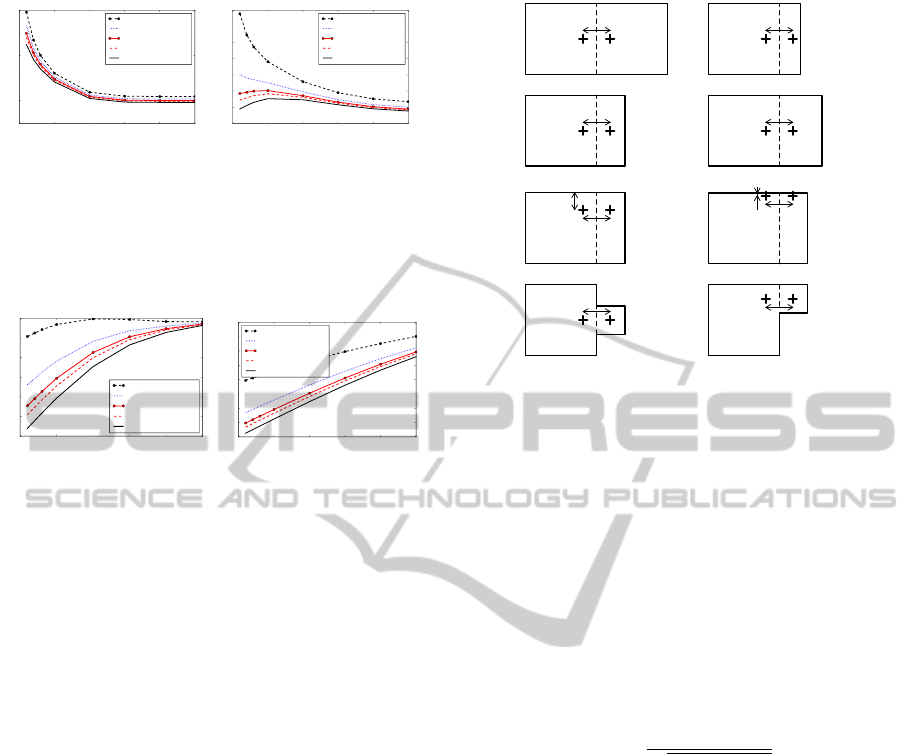
26x11 36x21 46x31 56x41 66x51
Area Size [px]
0.00
0.05
0.10
0.15
0.20
0.25
Diffusion Distance, t= 25
With Edge σ=0.4
With Edge σ=0.5
With Edge σ=0.6
With Edge σ=0.7
Without Edge σ=0.5
26x11 36x21 46x31 56x41 66x51
Area Size [px]
0.00
0.02
0.04
0.06
0.08
0.10
0.12
0.14
Diffusion Distance, t= 100
With Edge σ=0.4
With Edge σ=0.5
With Edge σ=0.6
With Edge σ=0.7
Without Edge σ=0.5
Figure 3: The dependence of diffusion distance on the area
size: The distance (vertical axis) is computed for the prob-
lem from Fig. 1 with/without the edge, for a = 15, and for
various values of t, σ, and for the increasing length of the
edge between the areas and for the increasing width of the
areas (both w and h are changing in this case). The value of
distance depends on the size.
0
5
10
15
20 25
a [px]
0.00
0.01
0.02
0.03
0.04
0.05
0.06
Diffusion Distance, t= 25
With Edge σ=0.4
With Edge σ=0.5
With Edge σ=0.6
With Edge σ=0.7
Without Edge σ=0.5
0
5
10
15
20 25
a [px]
0.000
0.005
0.010
0.015
0.020
0.025
0.030
0.035
0.040
Diffusion Distance, t= 100
With Edge σ=0.4
With Edge σ=0.5
With Edge σ=0.6
With Edge σ=0.7
Without Edge σ=0.5
Figure 4: The dependence of diffusion distance on the dis-
tance in the xy plane: The distance (vertical axis) is com-
puted for the problem from Fig. 1 with/without the edge,
for a constant image size (w = 50, h = 51), for various val-
ues of t, σ, and for the changing distance in the xy plane (the
value of a in pixels that is shown on the horizontal axis).
The value of diffusion distance depends on the value of a.
taken into account in the above mentioned simulation
(Fig. 1). Therefore, we created another set of test
cases to show that the diffusion distance depends on
the difference in size and on the mutual position of
the segments in which the points are placed. The set
is depicted in Fig. 5. We measure the diffusion dis-
tance between the points p and q lying in the areas
of various shapes. Two cases are considered for each
shape: (i) the points are placed in a single area, (ii)
the big area is split into two areas by inserting the
vertical splitting line (dashed line in Fig. 5); the dif-
ference of brightness between both areas is equal to 1.
The distance between p, q in the xy plane was a = 19
in all cases. Naturally, we would expect that the dis-
tances measured in the cases with two areas (with the
edge) will always be greater than the distances for the
cases with only one area. We could also hope that
the distances for all test cases with only one area will
remain more or less constant (similarly, for the test
cases with two areas). The computational simulation
showed that this is not always true. The resulting dis-
tances for each case are shown in Fig. 6. It can be seen
that the classical diffusion distance does not provide
the ordering in the sense that the distances measured
between the points lying in one image segment should
always be less than the distances measured between
the points lying in two different segments. It follows
p q
50 50
50
a=19
50 15
50
a=19
50 20
50
a=19
50 20
50
a=19
50 20
50a=19
12
50 20
50
a=19
2
50 20
15
20
15
a=19
50 20
20
15
a=19
Figure 5: Various configurations of image segments used
for testing the suitability of distance measuring methods.
The configurations presented here are referred to as case 1 -
8 in text.
that the value of distance does not give the informa-
tion that is needed for segmentation if we do not have
any apriori knowledge about the size of segments or
if the sizes may vary.
We also use this test set for evaluating the qual-
ity of measuring the distance and for comparing the
classical diffusion distance with the new measure that
is introduced in the next section. We introduce a dis-
criminative capability of distance measuring method,
which is defined by the following formula
D(t) =
|µ
e
(t) −µ
s
(t)|
p
σ
2
e
(t) + σ
2
s
(t)
, (10)
where µ
s
(t) and σ
2
s
(t) stand for the mean value and
variance, respectively, of the distance for the cases
without edge. Similarly, µ
e
(t), σ
2
e
(t) stand for the cor-
responding values for the cases with the edge. (We
note that the mentioned values are all dependent on
time.) The higher is the value of D(t), the better is
the method. The formula in Eq. (10) simply reflects
the fact that we would welcome if the distance mea-
sured for any case without edge were less than the dis-
tance measured for any case with edge. The compu-
tational simulation gave D (100) = 0.74 for the case
without noise (Fig. 6). The discriminative capabil-
ity shows the unsatisfactory behaviour of the classical
diffusion distance again. As can be seen, the intervals
corresponding to the cases with and without the edge
overlap each other, which says again that the diffusion
distance cannot distinguish between both cases.
For a certain visual illustration of the behaviour of
diffusion distance, we finally present an example in
Fig. 7. For a synthetic image with noise, the diffu-
ICPRAM2015-InternationalConferenceonPatternRecognitionApplicationsandMethods
124

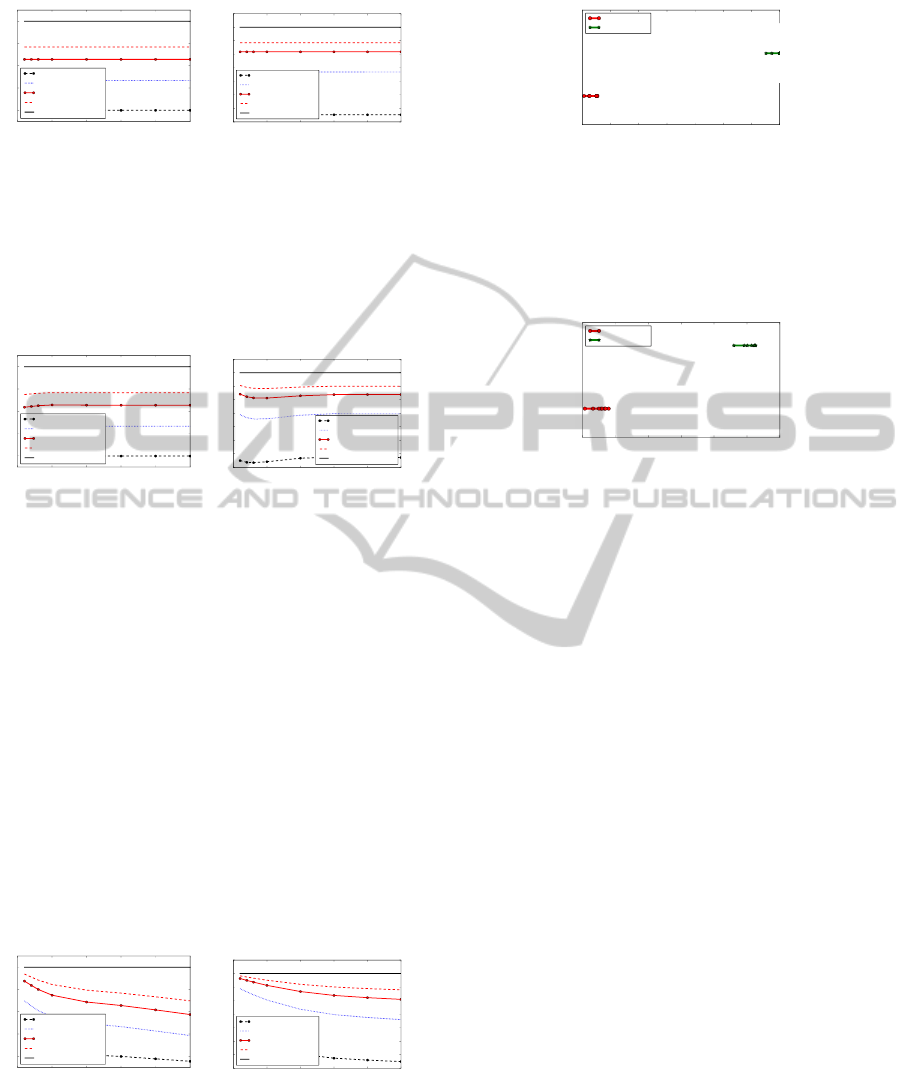
0.015 0.020 0.025 0.030 0.035 0.040
Distance
1
1
2
2
3
3
4
4
5
5
6
6
7
7
8
8
Diffusion Distance, t= 100
With Edge
Without Edge
Figure 6: Diffusion distance for various test cases from
Fig. 5 without noise, for the situation with and without the
edge, respectively, for t = 100, and σ = 0.5. The value of
discriminative capability is D(100) = 0.74 (µ
e
= 0.0294,
σ
2
e
= 0.31 ×10
−4
, µ
s
= 0.02398, σ
2
s
= 0.22 ×10
−4
).
Figure 7: For an image with noise (left image ), the diffu-
sion distances from the image centerpoint to all other pixels
are computed and depicted by brightness (right image); the
dark areas correspond to a small distance from the center-
point. Notice the highly changing distances inside the up-
per bright object area, especially, in the left part having the
shape of vertical strip. The distance step expected along the
boundary between the upper and lower object parts can be
better seen in the central area of the edge between the parts;
in the left area, the distance difference is less convincing.
sion distances from the image centerpoint to all other
pixels are computed. The parameters were set as fol-
lows. The ideal values of brightness were 0.0, 0.6, and
1.0, respectively. Gaussian noise with σ
n
= 0.075 was
added. The value of sigma from Eq. (3) was σ = 0.15.
The diffusion distance was computed for t = 250.
4 NORMALISED DIFFUSION
COSINE SIMILARITY
In this section, we propose an improvement that re-
duces the problems with the diffusion distance that
have been mentioned in the previous section. We
firstly define our approach. Then we explain why it
should be better than the diffusion distance.
For a given image, we introduce the diffusion co-
sine similarity between p, q at the time t as follows
s
t
(p,q) =
h
2t
(p,q)
p
h
2t
(p, p)h
2t
(q,q)
. (11)
By substitunig from Eq. (7), it can be easily seen that
s
t
(p,q) =
h~x
p
(t),~x
q
(t)i
p
h~x
p
(t),~x
p
(t)i
p
h~x
q
(t),~x
q
(t)i
=
h~x
p
(t),~x
q
(t)i
k~x
p
(t)kk~x
q
(t)k
. (12)
The value of s
t
(p,q) is equal to the value of the co-
sine of the angle between the vectors ~x
p
(t) and ~x
q
(t).
Since the value of h
t
(p,q) is always non-negative, the
value of s
t
(p,q) varies in the range of [0, 1].
To obtain a normalised cosine similarity, we eval-
uate the diffusion cosine similarity two times. Firstly,
for a given image. Secondly, for the corresponding
reference image, which is the image of the same size
as is the given input image, but with a constant bright-
ness everywhere. The normalised cosine similarity is
now the ratio between the similarity in the given im-
age and the similarity in the reference image. We note
that this ratio is only computed if the similarity in the
reference image is not close to zero. Otherwise, the
normalised cosine similarity is set to zero too, which
means that it cannot be computed reliably. Since the
diffusion cosine similarity in the given image is not
greater than the similarity in the reference image, the
maximal possible value of the normalised diffusion
cosine similarity is 1.
We should now explain why the normalised diffu-
sion cosine similarity is better than the diffusion dis-
tance. The reason is simple. The value of normalised
cosine similarity itself tells more clearly whether or
not two points are close one to another (i.e. belong
to one image segment). No other additional informa-
tion is needed. The value of 1.0 expresses the max-
imal possible concordance, decreasing values mean
increasing difference. We stress the following proper-
ties. The normalised cosine similarity is independent
on the length of the edge along which two areas touch
(see Fig. 8 and compare it with Fig. 2 for the dif-
fusion distance). The normalised cosine similarity is
much less dependent on the total size of area (see Fig.
9 and compare it with Fig. 3). The normalised co-
sine similarity is much less dependent on the distance
between the points in the xy plane (see Fig. 10 and
compare it with Fig. 4). Further results will be pre-
sented in the next section.
For completeness, it should be pointed out that the
idea of using the cosine similarity in a related area
is not completely new. In (Brand, 2005), the author
mentions the use of cosine similarity in the context of
maximizing satisfaction and profit and in connection
with the commute-time distance. The author, how-
ever, does not present similar analysis (focused on the
use in the area of image segmentation) as we do in
this paper. Neither he uses the normalisation.
5 EXPERIMENTAL RESULTS
We start with the tests using the synthetic images.
Then the tests with the real-life images are also pre-
NormalisedDiffusionCosineSimilarityandItsUseforImageSegmentation
125
30x11 30x21 30x31 30x41 30x51
Area Size [px]
0.2
0.4
0.6
0.8
1.0
Normalised Diffusion Cosine Similarity, t= 25
With Edge σ=0.4
With Edge σ=0.5
With Edge σ=0.6
With Edge σ=0.7
Without Edge σ=0.5
30x11 30x21 30x31 30x41 30x51
Area Size [px]
0.3
0.4
0.5
0.6
0.7
0.8
0.9
1.0
Normalised Diffusion Cosine Similarity, t= 100
With Edge σ=0.4
With Edge σ=0.5
With Edge σ=0.6
With Edge σ=0.7
Without Edge σ=0.5
Figure 8: The dependency of normalised diffusion cosine
similarity on the length of the edge between the areas: The
similarity (vertical axis) is computed for the problem from
Fig. 1 with/without the edge, for a = 15, and for various
values of t, σ, and for the increasing length of the edge be-
tween the areas (the value of h); the width of areas remains
constant. In contrast to the diffusion distance, the new sim-
ilarity does not depend on the edge length in this test envi-
ronment (compare with Fig. 2).
26x11 36x21 46x31 56x41 66x51
Area Size [px]
0.2
0.4
0.6
0.8
1.0
Normalised Diffusion Cosine Similarity, t= 25
With Edge σ=0.4
With Edge σ=0.5
With Edge σ=0.6
With Edge σ=0.7
Without Edge σ=0.5
26x11 36x21 46x31 56x41 66x51
Area Size [px]
0.3
0.4
0.5
0.6
0.7
0.8
0.9
1.0
Normalised Diffusion Cosine Similarity, t= 100
With Edge σ=0.4
With Edge σ=0.5
With Edge σ=0.6
With Edge σ=0.7
Without Edge σ=0.5
Figure 9: The dependency of normalised diffusion cosine
similarity on the area size: The similarity (vertical axis)
is computed for the problem from Fig. 1 with/without the
edge, for a = 15, and for various values of t, σ, and for the
increasing length of the edge between the areas and for the
increasing width of the areas (w and h are changing). The
dependence of similarity on the area size is much smaller
than in the case of diffusion distance (Fig. 3).
sented. As a first experiment, we evaluate the dis-
criminative capability introduced in Eq. (10) based
on computing the distance or similarity in various area
configurations (Fig. 5). For the diffusion distance, the
results have already been presented in Fig. 6. For the
new method, the values are stated in Fig. 11. Notice
that the intervals into which the values of normalised
diffusion cosine similarity fall for the cases with and
without the edge, respectively, do not overlap, which
makes the discriminative capability very good.
Naturally, the behaviour of every method is also
0
5
10
15
20 25
a [px]
0.2
0.4
0.6
0.8
1.0
Normalised Diffusion Cosine Similarity, t= 25
With Edge σ=0.4
With Edge σ=0.5
With Edge σ=0.6
With Edge σ=0.7
Without Edge σ=0.5
0
5
10
15
20 25
a [px]
0.3
0.4
0.5
0.6
0.7
0.8
0.9
1.0
Normalised Diffusion Cosine Similarity, t= 100
With Edge σ=0.4
With Edge σ=0.5
With Edge σ=0.6
With Edge σ=0.7
Without Edge σ=0.5
Figure 10: The dependency of normalised diffusion cosine
similarity on the distance in the xy plane: The similarity
(vertical axis) is computed for the problem from Fig. 1
with/without the edge, for a constant image size (w = 50,
h = 51), for various values of t, σ, and for the increasing
distance in the xy plane (the value of a on the horizontal
axis). Due to the normalisation, the similarity depends on a
much less than the diffusion distance (Fig. 4).
0.65 0.70 0.75 0.80 0.85 0.90 0.95 1.00
Similarity
1
1
2
2
3
3
4
4
5
5
6
6
7
7
8
8
Normalised Diffusion Cosine Similarity, t= 100
With Edge
Without Edge
Figure 11: Normalised diffusion cosine similarity for the
test cases from Fig. 5 without noise, for the situation with
and without edge, respectively, for t = 100, and σ = 0.5.
The value of discriminative capability is D(100) = 26.9
(µ
e
= 0.669, σ
2
e
= 0.71 ×10
−4
, µ
s
= 0.995, σ
2
s
= 0.75 ×
10
−4
), which is a substantial improvement in comparison
to the value for the diffusion distance shown in Fig. 6.
0.60 0.65 0.70 0.75 0.80 0.85 0.90
Similarity
1
1
2
2
3
3
4
4
5
5
6
6
7
7
8
8
Normalised Diffusion Cosine Similarity, t= 100
With Edge
Without Edge
Figure 12: Normalised diffusion cosine similarity for the
same situation as in Fig. 11, but with the Gaussian noise
σ
n
= 0.2 added to the test images. The resulting discrim-
inative capability is D (100) = 4.164 (µ
e
= 0.626, σ
2
e
=
0.234 ×10
−2
, µ
s
= 0.854, σ
2
s
= 0.651 ×10
−3
), which still
is better than the value for the diffusion distance without
noise.
important in the presence of noise. We carried out the
same test for the noisy images too. Gaussian noise
was added to all test images (Fig 5). For each test
image, 1000 samples were used in simulation (see
Fig. 12 for further details). Even with a relatively
big amount of noise, the results of the new method
were better (Fig. 12) then the results obtained for the
diffusion distance without noise.
As a further example, we also present the result
for the image from Fig. 7. The normalised diffusion
cosine similarity is depicted in Fig. 13. The similar-
ity is measured between the image center point and all
remaining pixels and is depicted as brightness. Since
big similarity corresponds to a small distance, we also
present an inverse image for more convenient compar-
ison with the result for diffusion distance (Fig. 7). Al-
though we do not present any quantitative evaluation
in this case, we believe that the result of the new sim-
ilarity may be regarded as visually better (Fig. 13).
In the rest of this section, we focus on the real-life
images and their seeded (interactive) segmentation
(Sinop and Grady, 2007). For this purpose, the sim-
ilarity (proximity) between the pixel and area should
be defined. Let
∑
top
Q
{collection} stand for the sum
of the biggest Q elements from a collection of real
numbers. The normalised diffusion cosine proximity,
denoted by ˜s
t
(p,A), between a point p and an area A
ICPRAM2015-InternationalConferenceonPatternRecognitionApplicationsandMethods
126

Figure 13: The value of the normalised diffusion cosine
similarity between the image center point and all remaining
pixels is computed under exactly the same conditions as in
Fig. 7 for the diffusion distance. In the left image, the simi-
larity is depicted by brightness (the bright places indicate a
high similarity). For more convenient comparison with the
result for the diffusion distance, also the inverse image is
presented (right image).
can be introduced by the formula
˜s
t
(p,A) =
1
Q
∑
top
Q
{˜s
t
(p,q)}
q∈A
. (13)
The formula simply reflects the fact that p and A may
be regarded as close if at least a certain number of
points exist in A that are close to p. The formula can
also be easily adapted for the diffusion distance (in-
stead of the Q points with the biggest similarities, Q
points with the smallest distances are considered).
We note that the segmentation algorithm itself is
not the direct focus of our work, i.e. we do not pro-
pose a new algorithm. Instead, by making use of a
certain algorithm, we demonstrate the properties of
the new similarity measure that might be useful in var-
ious known or future algorithms based on measuring
the distance or similarity. The algorithm used for test-
ing should make it possible to present the properties
of the new measure clearly; understanding the results
should not be made more difficult due to the proper-
ties of algorithm. For this reason, we use the simple
one-step seeded segmentation.
The seeds of the objects and the background are
defined manually. Once it is done, the distance to the
seeds is computed for all remaining image pixels. If
the distance of a pixel is lower to the object seed than
to the background seed, the pixel is marked as an ob-
ject pixel. Otherwise, it is marked as a background
pixel. The algorithm can be easily adapted for the use
of similarity instead of distance.
Several real-life images from the Berkeley Seg-
mentation Dataset (Martin et al., 2001) were used
(Fig. 14) and processed as follows. The conversion
to greyscale was carried out, which was followed by
the normalisation of intensity values into the interval
[0,1]. The normalised images were slightly filtered by
making use of anisotropic diffusion filtering; the fil-
tered images used for further processing are shown in
Fig. 14 too. For all images, we used σ = 0.07 (Eq. 3),
t = 150, Q = 10, and 750 eigenvectors. The size of
images was 160 ×240 pixels. The suitable values of
t and Q were determined experimentally on the basis
of visual evaluation of the results. For the diffusion
distance as well as for the new similarity, the best re-
sults were obtained for 100 ≤ t ≤ 200, 4 ≤ Q ≤ 50.
The results of the segmentation using the new nor-
malised diffusion cosine similarity, the diffusion dis-
tance, and the cosine similarity mentioned in (Brand,
2005) are shown in Fig. 14. It can be seen that the
new similarity gives visually better results than the
remaining mentioned measures. Naturally, all the re-
sults could be improved by modifying the position of
the seeds. However, we did not do so since we wanted
to show the properties of the distance/similarity mea-
sures clearly.
Finally, we note that we did not aim at compar-
ing the above segmentation algorithms with all other
main state-of-the-art approaches. Instead, we used
them to show that the theoretical findings and expec-
tations presented before are correct and useful for the
practice (see the conclusion for the discussion about
our main goals and contributions).
6 CONCLUSIONS
Measuring the distances along the surface that is de-
fined by the image function seems to be useful in
more complicated situations. The use of geodesic dis-
tance is often mentioned in this context, but its disad-
vantages are known. One would intuitively say that
the diffusion distance should have good properties
for the mentioned purpose. We showed (including
the computational simulations of the situations that
are important for segmentation) that the diffusion dis-
tance need not be useful since the presence of edges
may be overshadowed by the varying size of image
segments (and the size is not often known in advance).
We proposed a new measure called normalised diffu-
sion cosine similarity that suffers from these problems
to a much lesser extent. We have also demonstrated
that it can be used in image segmentation algorithms.
We believe that the geodesic distance and diffu-
sion distance (resistance or commute-time distance)
are two opposite approaches. While the geodesic dis-
tance only searches for the shortest path between the
points, the diffusion distance takes into account all
possible paths. The idea of simultaneously examining
more paths seems to be generally useful. The ques-
tion, however, remains how it should be exactly done.
The diffusion distance does not seem to be the best
solution. We believe that a certain gap exists in this
area and that the corresponding efficient methods will
probably be developed in the future. We intended this
paper as a certain step in this direction rather than a
paper proposing a new segmentation method for ev-
NormalisedDiffusionCosineSimilarityandItsUseforImageSegmentation
127

Figure 14: One-step seeded segmentation: The source im-
ages (the first row); the seeds for the objects and the back-
ground (the second row); the filtered images that were used
for further processing (the third row); the normalised diffu-
sion cosine similarity of pixels to the object seeds, the bright
areas correspond to a high similarity (the fourth row); the
objects extracted by making use of the new similarity (the
fifth row); the diffusion distance from the object seeds, the
dark areas correspond to a small distance (the sixth row); the
objects extracted by making use of the diffusion distance
(the seventh row); the objects extracted by making use of
the cosine similarity mentioned in (Brand, 2005) (the last
row).
eryday use. That is why we did not aim at comparing
the algorithm mentioned in the previous section with
various other state-of-the-art algorithms. The goal
was to show that some alternatives exist in the area of
the diffusion-like distances that may have a chance to
be developed into useful and practical tools. We hope
that introducing the new normalised diffusion cosine
similarity can be regarded as a step in this direction.
ACKNOWLEDGEMENTS
This work was partially supported by the grant of SGS
No. SP2014/170, V
ˇ
SB - Technical University of Os-
trava, Czech Republic.
REFERENCES
Babi
´
c, D., Klein, D. J., Lukovits, I., Nikoli, S., and Trina-
jsti, N. (2002). Resistance-distance matrix: A com-
putational algorithm and its application. International
Journal of Quantum Chemistry, 90(1):166–176.
Brand, M. (2005). A random walks perspective on maxi-
mizing satisfaction and profit. In Proceedings of the
2005 SIAM International Conference on Data Mining,
pages 12–19. SIAM.
Coifman, R. R. and Lafon, S. (2006). Diffusion
maps. Applied and Computational Harmonic Anal-
ysis, 21(1):5–30.
Eppstein, D. (1998). Finding the k shortest paths. SIAM J.
Computing, 28(2):652–673.
Fouss, F., Pirotte, A., Renders, J.-M., and Saerens, M.
(2007). Random-walk computation of similarities be-
tween nodes of a graph with application to collabo-
rative recommendation. IEEE Trans. on Knowl. and
Data Eng., 19(3):355–369.
Grady, L. (2006). Random walks for image segmentation.
IEEE Trans. Pattern Anal. Mach. Intell., 28(11):1768–
1783.
Huang, H., Yoo, S., Qin, H., and Yu, D. (2011). A robust
clustering algorithm based on aggregated heat kernel
mapping. In Cook, D. J., Pei, J., 0010, W. W., Zaane,
O. R., and Wu, X., editors, ICDM, pages 270–279.
IEEE.
Klein, D. J. and Randi
´
c, M. (1993). Resistance distance.
Mathematical Chemistry, 12(1):81–95.
Lafon, S. and Lee, A. B. (2006). Diffusion maps and coarse-
graining: A unified framework for dimensionality re-
duction, graph partitioning and data set parameteriza-
tion. IEEE Transactions on Pattern Analysis and Ma-
chine Intelligence, 28:1393–1403.
Lipman, Y., Rustamov, R. M., and Funkhouser, T. A.
(2010). Biharmonic distance. ACM Trans. Graph.,
29(3):27:1–27:11.
Martin, D., Fowlkes, C., Tal, D., and Malik, J. (2001). A
database of human segmented natural images and its
ICPRAM2015-InternationalConferenceonPatternRecognitionApplicationsandMethods
128

application to evaluating segmentation algorithms and
measuring ecological statistics. In in Proc. 8th Intl
Conf. Computer Vision, pages 416–423.
Nadler, B., Lafon, S., Coifman, R. R., and Kevrekidis, I. G.
(2005). Diffusion maps, spectral clustering and eigen-
functions of fokker-planck operators. In in Advances
in Neural Information Processing Systems 18, pages
955–962. MIT Press.
Papadimitriou, C. H. (1985). An algorithm for shortest-path
motion in three dimensions. Information Processing
Letters, 20(5):259 – 263.
Qiu, H. and Hancock, E. R. (2007). Clustering and embed-
ding using commute times. IEEE Trans. Pattern Anal.
Mach. Intell., 29(11):1873–1890.
Sharma, A., Horaud, R., Cech, J., and Boyer, E. (2011).
Topologically-Robust 3D Shape Matching Based on
Diffusion Geometry and Seed Growing. In CVPR ’11
- IEEE Conference on Computer Vision and Pattern
Recognition, pages 2481–2488, Colorado Springs,
United States. IEEE Computer Society Press.
Sinop, A. K. and Grady, L. (2007). A seeded image seg-
mentation framework unifying graph cuts and random
walker which yields A new algorithm. In IEEE 11th
International Conference on Computer Vision, ICCV
2007, Rio de Janeiro, Brazil, October 14-20, 2007,
pages 1–8. IEEE.
Surazhsky, V., Surazhsky, T., Kirsanov, D., Gortler, S. J.,
and Hoppe, H. (2005). Fast exact and approximate
geodesics on meshes. ACM Trans. Graph., 24(3):553–
560.
Tenenbaum, J. B., de Silva, V., and Langford, J. C. (2000).
A global geometric framework for nonlinear dimen-
sionality reduction. Science, 290(5500):2319.
von Luxburg, U., Radl, A., and Hein, M. (2014). Hit-
ting and commute times in large random neighbor-
hood graphs. Journal of Machine Learning Research,
15:1751–1798.
Yen, L., Fouss, F., Decaestecker, C., Francq, P., and
Saerens, M. (2007). Graph nodes clustering based
on the commute-time kernel. In Proceedings of the
11th Pacific-Asia Conference on Advances in Knowl-
edge Discovery and Data Mining, PAKDD’07, pages
1037–1045, Berlin, Heidelberg. Springer-Verlag.
NormalisedDiffusionCosineSimilarityandItsUseforImageSegmentation
129
