Mixed Integer Programming with Decomposition to Solve a Workforce

Scheduling and Routing Problem

Wasakorn Laesanklang, Dario Landa-Silva and J. Arturo Castillo-Salazar

School of Computer Science, ASAP Research Group, The University of Nottingham, Nottingham, U.K.

Keywords:

Workforce scheduling, Routing problem, Home care scheduling, Mixed integer programming, Problem

decomposition.

Abstract:

We propose an approach based on mixed integer programming (MIP) with decomposition to solve a workforce

scheduling and routing problem, in which a set of workers should be assigned to tasks that are distributed

across different geographical locations. This problem arises from a number of home care planning scenarios

in the UK, faced by our industrial partner. We present a mixed integer programming model that incorporates

important real-world features of the problem such as deﬁned geographical regions and ﬂexibility in the workers’

availability. Given the size of the real-world instances, we propose to decompose the problem based on

geographical areas. We show that the quality of the overall solution is affected by the ordering in which the

sub-problems are tackled. Hence, we investigate different ordering strategies to solve the sub-problems and

show that such decomposition approach is a very promising technique to produce high-quality solutions in

practical computational times using an exact optimization method.

1 INTRODUCTION

The workforce scheduling and routing problem

(WSRP) is a difﬁcult problem that arises in industries

like home care, health care, patrol service, meter read-

ing, etc. (Castillo-Salazar et al., 2014). One speciﬁc

example of WSRP is home health care services where

nurses or care workers should deliver care services

at the patient’s home. Solving the problem involves

producing a job schedule and a route for each worker

while satisfying the business requirements and consid-

ering workers qualiﬁcations and skills, task require-

ments, travelling distances, etc. It is usually expected

that the solution gives the lowest operational cost.

Developing automated solution methods to solve

WSRP scenarios is a current research challenge as

reﬂected by recent published research (Mankowska

et al., 2014; Liu et al., 2014; Hart et al., 2014). Solv-

ing an instance of WSRP often requires the expertise

and knowledge of a human planner (Barrera et al.,

2012). In this research, we are working with an in-

dustrial partner who provides scheduling services for

businesses and other organisations facing this type of

problems. The data sets considered here come from

real-world scenarios. A particular feature is that ‘work-

ing areas’ or ‘regions’ are pre-deﬁned and this affects

the difﬁculty of the problem being tackled.

Tackling WSRP with exact optimization methods

to produce solutions in practice is still a research chal-

lenge. Since obtaining an optimal schedule is the

ultimate goal, exact methods like mathematical pro-

gramming are a suitable approach. However, proven

optimality with exact methods has been shown mainly

on problem instances of limited size (Borsani et al.,

2006; Bredstrom and Ronnqvist, 2007). Problem in-

stances faced in practice are larger and for solving

them, heuristic methods are usually considered more

efﬁcient in terms of computation time (Akjiratikarl

et al., 2007; Pillac et al., 2012). The motivation for our

work is to develop a solution approach based on exact

optimization to tackle real-world WSRP instances.

In this paper, we propose a decomposition ap-

proach that uses mixed integer programming to tackle

WSRP instances of practical size. The proposed

method splits the problem into sub-problems according

to deﬁned geographical areas. Our computational ex-

periments show that the approach allows to explore the

trade-off between computation efﬁciency and solution

quality. Moreover, the insights from our experiments

suggest that success of decomposition varies accord-

ing to the problem instance, which provides us with

ideas for future research.

The main contribution of this paper is to show

that the ordering in which sub-problems in workforce

283

Laesanklang W., Landa-Silva D. and Arturo Castillo Salazar J..

Mixed Integer Programming with Decomposition to Solve a Workforce Scheduling and Routing Problem.

DOI: 10.5220/0005223602830293

In Proceedings of the International Conference on Operations Research and Enterprise Systems (ICORES-2015), pages 283-293

ISBN: 978-989-758-075-8

 2015 SCITEPRESS (Science and Technology Publications, Lda.)

scheduling and routing are tackled within a decompo-

sition approach, has an effect on the computational

efﬁciency and achieved solution quality. Following

this, some ordering strategies are proposed to achieve

solutions of good quality, typically 16.36% of relative

gap on average, in practical computation time.

Section 2 reviews related works in the literature and

establishes the motivation for the research in this paper.

Section 3 gives the problem deﬁnition and formulation

for the WSRP considered here. Section 4 describes

the proposed MIP with decomposition approach and

the experimental study, including description of test

data instances. The ﬁnal section summarises the paper

and outlines some of the proposed future work.

2 LITERATURE REVIEW

Solving integer programming formulations for larger

problem instances still has its limitations in terms of

computation time. Mathematical programming has

been used in the literature to tackle some WSRP. Exam-

ples include linear programming (Angelis, 1998), inte-

ger programming (Kergosien et al., 2009) and mixed

integer programming (Bredstrom and Ronnqvist, 2007;

Dohn et al., 2009; Borsani et al., 2006; Rasmussen

et al., 2012). Solving real-world size problems often

resources to heuristic or hybrid algorithms (Bertels

and Torsten, 2006; Akjiratikarl et al., 2007; Eveborn

et al., 2009). There are some improved exact meth-

ods, like branch and price (Bredstrom and Ronnqvist,

2007; Dohn et al., 2009; Rasmussen et al., 2012), that

can deal with large instances. Branch and price re-

quires problem reformulation which usually involves

Dantzig-Wolfe decomposition to compute a tighter re-

laxation bound (Vanderbeck, 2000; Feillet, 2010). The

algorithm also requires two steps to repeatedly solve

the problem in order to improve the solution.

Decomposition techniques are another good alter-

native to apply exact optimization methods to large in-

teger programming formulations. The basic idea here

is to transform or split the problem into smaller sub-

problems. This technique has been applied in various

problem domains. For example, Benders’ decomposi-

tion was used to produce solutions for large instances

of the aircraft routing and crew scheduling problem

(Cordeau et al., 2001; Mercier et al., 2005). Benders’

decomposition is suitable for problems with exclu-

sive sub-problem sets or problems that shows some

block structures linked by constraints (Benders, 1962).

In another example (Perl and Daskin, 1985) split the

warehouse location-routing problem into three smaller

problems: the complete multi-depot vehicle-dispatch

problem, the warehouse location-allocation problem

and the multi-depot routing-allocation problem. These

three smaller problems were solved in phases and each

of them was formulated with mathematical program-

ming and solved by an exact solver. For detailed re-

views of decomposition approaches see (Ralphs and

Galati, 2010; Vanderbeck and Wolsey, 2010).

Decomposition techniques have also been applied

within heuristic approaches using some form of clus-

tering. For example, (Reimann et al., 2004) tackled

a large vehicle routing problem by decomposing it

into sub-problems. Each sub-problem was a cluster of

customers assigned to a vehicle which then became a

travelling salesman problem. The sub-problem size is

controlled by splitting a large sub-problem to shrink

the corresponding cluster. Similar ideas were applied

in a hybrid heuristic for generating multi-carrier trans-

portation plans (Landa-Silva et al., 2011).

The purpose of this paper is to propose a decompo-

sition approach that uses mixed integer programming

(MIP) to tackle workforce scheduling and routing prob-

lem instances arising in real-world scenarios. For this,

we also present an MIP formulation that incorporates

features of the WSRP scenarios faced by our indus-

trial partner. The proposed decomposition technique

does not require some formulation structure like in

Benders’ decomposition neither uses a heuristic solver.

Our approach harness the power of exact optimization

solvers while decomposing the problem instances in a

way that is meaningful to practice.

3 PROBLEM DESCRIPTION AND

FORMULATION

The goal in WSRP is to assign each worker to under-

take a set of tasks across a set of geographical loca-

tions. A path is the series of tasks to be performed by

a worker within the planning period. A good quality

solution consists of a set of shortest paths represent-

ing the task assignments for each worker at the lowest

cost. The solution should also respect other conditions

such as task pre-requisites, required travelling time be-

tween locations, deﬁned appointment times, workers’

skills, workers availability, restricted working regions,

working time limits, etc.

Consider a graph

G = (V, E)

where

V = T ∪ D ∪

represents the union of a set of tasks (each task

as a location)

, a set of start locations

and a set

of end locations

while

represents a set of links

between two locations (e.g. between two task locations

or between the worker’s home and a task location).

The set of workers is denoted by

. Binary decision

variable

i, j

= 1

if worker

c ∈ C

is assigned to a task

j ∈ T

after ﬁnishing task

i ∈ T

i, j

= 0

otherwise.

ICORES2015-InternationalConferenceonOperationsResearchandEnterpriseSystems

284

Note that elements of

are referred here as tasks but

also each task has an associated location.

In practical scenarios like the ones considered here,

the available workforce and its skills are often not

sufﬁcient to cover all the tasks that need performing.

This can be addressed by introducing a dummy worker

(through a binary decision variable

) that takes any

excess work that cannot be assigned to the real work-

force (Bredstrom and Ronnqvist, 2008; Rasmussen

et al., 2012). Then, the assignment of tasks is repre-

sented by (1).

∑

c∈C

∑

i∈D∪T

i, j

+ y

= 1 , ∀ j ∈ T (1)

The sequence of tasks that a worker performs is

represented as a path for visiting task locations, hence

the number of workers arriving at one location must be

equal to the number of workers leaving that task loca-

tion so that either workers are assigned to the next task

or go home. Then, the path constraint is represented

by (2).

∑

i∈D∪T

i, j

∑

k∈D

∪T

j,k

, ∀ j ∈ T, ∀c ∈ C (2)

Workers must start and end their paths from their

speciﬁc location (e.g. their home or a central ofﬁce) as

given by (3) and (4). Since

and

are sets of start

and end locations respectively, these two constraints

indicate the start and end locations for each worker.

Also, workers leave their start location and enter their

end location at most once (although the start and end

locations can be different) as expressed by (5) and

(6) respectively. Note that a worker does not leave

his start location if he is not assigned to work. This

is different from the common case in the literature

where all workers leave their start location. In our

problem instances, the speciﬁc start and end locations

are provided for every worker.

∑

j∈D

∪T

k, j

≥

∑

j∈D

∪T

i, j

, ∀c ∈ C, ∀i ∈ T, ∃k ∈ D (3)

∑

i∈D∪T

i,k

≥

∑

i∈D∪T

i, j

, ∀c ∈ C, ∀ j ∈ T, ∃k ∈ D

(4)

∑

j∈D

∪T

i, j

≤ 1 , ∀i ∈ D, ∀c ∈ C (5)

∑

i∈D∪T

i, j

≤ 1 , ∀ j ∈ D

, ∀c ∈ C (6)

Let

be the set of skills and

s ∈ S

a particular

skill. For worker

the qualiﬁcation level on skill

and for task

the requirement of skill

s, j

Hence, worker

can be assigned to task

only if the

worker has the required qualiﬁcations level for skill

, that is,

≥ r

s, j

. Then, in our model the multi-skill

qualiﬁcation requirements are represented by (7).

i, j

s, j

≤ q

, ∀c ∈ C, ∀i ∈ D ∪T, ∀ j ∈ T, ∀s ∈ S (7)

Also, travel time between task locations must be

feasible. Decision variable

takes a positive frac-

tional value that gives the worker arrival time to the

location of task

. Note that the maximum arrival time

value is 1440 which is equivalent to the 24

hour of

the day. Let

be the arrival times of worker

the locations of task

and task

respectively. Let

i, j

be the travelling time between the locations of tasks

and

. Let

be the duration of task

. Then, if worker

is assigned to perform task

after completing task

inequality (8) (

is a large constant number) expresses

the arrival on time requirement.

+ M(1 − x

i, j

) ≥ a

+ x

i, j

+ δ

, ∀c ∈ C, ∀i ∈ D ∪T, ∀ j ∈ D

∪ T (8)

An arrival time window is also deﬁned for task

and

the worker should not arrive earlier than

or later

than w

, as expressed by (9).

≤ a

≤ w

, ∀i ∈ T, ∀c ∈ C (9)

An important feature of our WSRP scenarios is

that working regulations and availability can be spe-

ciﬁc for each worker. In the problems considered here,

this refers to long breaks between shifts (short breaks

within the working shift are not considered), days-

off, working shift duration, maximum working hours,

and speciﬁc worker preferences (e.g. late morning,

afternoon only, whole day, overnight). We adopt a

ﬂexible availability constraint from an optimization of

daily scheduling for home health care services (Traut-

samwieser and Hirsch, 2011). Any task assignment

at time

including the task duration

should lie in

between the shift starting time

and the shift end-

ing time

. The availability parameters

and

are real numbers deﬁned for each worker

. A task

assigned outside the shift is charged as additional ex-

pense, hence binary decision variable

= 1

if this is

the case and

= 0

otherwise. Then, individual avail-

ability constraints are denoted by (10) and (11) while

the working hours limit (

) constraint is denoted by

(12).

− a

≤ M(1 − x

i, j

+ ω

)

∀c ∈ C, ∀i ∈ D ∪ T, ∀ j ∈ T (10)

MixedIntegerProgrammingwithDecompositiontoSolveaWorkforceSchedulingandRoutingProblem

285

+ δ

− α

≤ M(1 − x

i, j

+ ω

)

∀c ∈ C, ∀i ∈ D ∪ T, ∀ j ∈ T (11)

∑

i∈D∪T

∑

j∈T

i, j

≤ h

, ∀c ∈ C (12)

Another important feature of our WSRP scenar-

ios is that workers have preferred geographical areas

for working but the decision maker can still request

workers to work outside those preferred regions. We

formulate this in (13) where binary parameter

= 1

if worker

is willing and able to work at the location

of task

= 0

otherwise, and binary decision vari-

able

= 1

if worker

is forced to work outside their

deﬁned regions.

∑

i∈D∪T

i, j

− ψ

≤ γ

, ∀c ∈ C, ∀ j ∈ T (13)

Most of the above constraint formulations exist in

literature but not all. Common constraints (see also

(Castillo-Salazar et al., 2014)) such as path constraint

(2), skill and qualiﬁcation (7) and time windows (9)

form the basic structure of the scheduling and routing

problem (Dantzig and Ramser, 1959; Bredstrom and

Ronnqvist, 2008; Dohn et al., 2009; Castro-Gutierrez

et al., 2011; Rasmussen et al., 2012). Tailor cut con-

straints adopted from literature are the availability con-

straints (10,11) while the constraints that required fur-

ther adaptation to our problem features are the working

region (13) (implemented as soft constraint) and start-

end paths (3-6).

Table 1 summarises the constraints in our MIP

model. Given our real-world data sets, some are im-

plemented as soft constraints. For example, workers

can be forced to work outside their predeﬁned regions

and availability. Also, tasks can be left unassigned

(assigned to the dummy worker). These features are

quite important to maintain the practical applicability

of our model and solution approach.

The objective function (14) involves three costs:

monetary cost, preferences penalty cost and soft con-

straints penalty cost.

Min

∑

c∈C

∑

i∈D∪T

∑

j∈D

∪T



i, j

+ p



i, j

∑

c∈C

∑

i∈D∪T

∑

j∈D

∪T

i, j

∑

j∈T

+ M

(ω

+ ψ

) (14)

The ﬁrst term in (14) is the monetary cost and in-

cludes the travelling cost

i, j

of going from location of

task

to the location of task

, and the payment

for

Table 1: Summary of problem requirements and type of

constraints.

Hard Soft

Job assignment (Cons. (1)) *

Path constraint (Cons. (2)) *

Start-end paths (Cons. (3) - (6)) *

Skill and qualiﬁcation (Cons. (7)) *

Travel time feasibility (Cons. (8)) *

Time windows (Cons. (9)) *

Worker availability (Cons. (10),(11)) † *

Working hours limit (Cons. (12)) *

Working regions (Cons. (13)) *

†

Hard constraints (15) and (16) are described in Sec-

tion 4.2 and only apply to the decomposition model.

worker

to perform task

. The second term in (14) is

the preference penalty cost denoted by

≥ 0

and is a

summation of penalties for not meeting worker-client

preferences, required skill preferences and working

region preferences. This penalty value can go from 0

to 75 and

= 0

when all preferences are met, while

this penalty value grows higher as the preference level

of assigning worker

to task

decreases. The third

term in (14) is the soft constraints penalty cost due

to the violation of the three soft constraints in the

model. The job assignment constraint has the highest

priority (

= 2000

), so a violation of this constraint

type costs more than a violation of the the other two

constraints. The worker availability and working re-

gions constraints have the same priority (

= 500

Note that the working regions constraint is involved

in two costs. If the worker is assigned a task in a

non-preferred region then this is a constraint penalty

cost. If the worker is assigned to one of the preferred

regions this is quantiﬁed as a preference penalty cost

according to the degree in which the region is preferred

by the worker (several working regions with different

preference levels).

The above MIP model corresponds to the inte-

grated scheduling and routing problem. Solving this

model with an exact optimization method is not prac-

tical considering our real-world problem instances.

Hence, we apply a decomposition technique.

4 DECOMPOSITION APPROACH

AND STUDY

In order to reduce the overall computational time of

solving real-world instances of the integrated work-

force scheduling and routing problem, we propose a

decomposition method in this section. First, we de-

scribe the features of our problem instances as this will

help to explain the proposed decomposition approach.

ICORES2015-InternationalConferenceonOperationsResearchandEnterpriseSystems

286

Later, the method is described and experimental results

are presented.

4.1 Test Instances

For the present work, we prepared some test instances

using real-world data corresponding to home care sce-

narios in the UK, provided by our industrial partner.

A problem instance

has a set of locations

. Recall

from Section 3 that

V = D ∪ T ∪ D

. Also, some of the

tasks

{ j

, j

, . . . , j

}

share the same geographi-

cal location

κ ∈ K

, where

is a set of geographical

locations. A group of locations are assembled as a

geographical area or working region

a ∈ A

. Note that

a ⊆ K

and

is a partition. Also, an individual worker

may work on one or several geographical areas. As

noted above, a key aspect of our scenarios is that sev-

eral tasks might be required at one particular location.

Each individual task may have different required skills,

worker preferences and worker cost.

We took four real-world scenarios and prepared

a data set from each. Although the instances in each

data set come from the same scenario, each instance

is formed from a different planning time giving a vari-

ation in the available human resources and task re-

quirements. In our data, the start and end locations

of a worker are the same (

d = d

). Table 2 shows the

main features of the test instances: the number of avail-

able workers

|C|

, the number of task locations

|K|

, the

numbers of tasks

|T |

and the number of predeﬁned

geographical areas

|A|

. In terms of size, instances

WSRP-A-(01-07) and WSRP-B-(01-07) are consid-

ered small with around 19-34 workers and 13-69 tasks.

The optimal solution for each of these instances can be

found in less than 5 minutes. Instances WSRP-D-(01-

07) and WSRP-F-(01-07) are considered large with

more than 100 workers and 400 tasks. These large in-

stances cannot yet be solved to optimality in practical

computation time. In our experimental study, we use

the small instances to validate the proposed decom-

position approach as we can compare to the optimal

solutions. Moreover, the experimental results show the

suitability of the decomposition approach in tackling

the large instances using an exact optimization solver.

4.2 Geographical Decomposition with

Conﬂict Avoidance

In this paper, the workforce scheduling and routing

problem is decomposed into working regions as this is

a key feature of the scenarios provided by our indus-

trial partner. Since we decompose the problem into

sub-problems to deal with the larger size more efﬁ-

ciently, by solving the sub-problems one at a time in

Table 2: The test data sets.

Instance |C| |K| |T | |A|

WSRP-A-01 23 25 31 6

WSRP-A-02 22 24 31 4

WSRP-A-03 22 28 38 5

WSRP-A-04 19 22 28 3

WSRP-A-05 19 9 13 3

WSRP-A-06 21 22 28 7

WSRP-A-07 21 9 13 3

WSRP-B-01 25 27 36 6

WSRP-B-02 25 11 12 4

WSRP-B-03 34 43 69 6

WSRP-B-04 34 14 30 4

WSRP-B-05 32 38 61 8

WSRP-B-06 32 38 57 7

WSRP-B-07 32 38 61 7

WSRP-D-01 164 233 483 13

WSRP-D-02 166 215 454 12

WSRP-D-03 174 279 585 15

WSRP-D-04 174 237 520 15

WSRP-D-05 173 259 538 15

WSRP-D-06 174 291 610 15

WSRP-D-07 173 293 611 15

WSRP-F-01 805 477 1211 45

WSRP-F-02 769 496 1243 46

WSRP-F-03 898 582 1479 54

WSRP-F-04 789 513 1448 47

WSRP-F-05 883 626 1599 59

WSRP-F-06 783 565 1582 44

WSRP-F-07 1011 711 1726 64

|C| = number of workers.

|K| = number of task locations.

|T | = number of required tasks.

|A| = number of working regions.

a given sequence, we can no longer guarantee overall

optimality.

Basically, the decomposition method generates a

sub-problem for each working region and solves each

sub-problem in sequence. Worker assignment con-

ﬂicts (i.e. a worker being assigned to different task

locations at the same time) are avoided because each

sub-problem is solved using only the reduced available

workforce after solving the previous sub-problem.

Algorithm 1 presents the proposed geographi-

cal decomposition with conﬂict avoidance approach

(GDCA). A problem instance

is split into several sub-

problems

(step 2). A sub-problem

corresponds to

a geographical area or working region

a ∈ A

. Then, the

sub-problems are solved in a given sequence (steps 3-

6) and different solving sequences can lead to different

solution quality. This is because the ﬁrst sub-problem

has access to the most workforce resources but subse-

quent sub-problems will have access to limited avail-

able workforce. Since worker assignment conﬂicts

are avoided, this means that the hard constraints ex-

MixedIntegerProgrammingwithDecompositiontoSolveaWorkforceSchedulingandRoutingProblem

287

pressed by equations (15) and (16) are enforced in this

algorithm.

+ δ

− β

≤ M(2 − x

i, j

− ζ

)

∀c ∈ C, ∀i ∈ D ∪ T, ∀ j ∈ T ∪ D

(15)

− a

≤ M(1 − x

i, j

+ ζ

)

∀c ∈ C, ∀i ∈ D ∪ T, ∀ j ∈ T ∪ D

(16)

Here,

denotes the start of unavailable time and

denotes the end of unavailable time for worker

Since the original model generates a continuous path

for a worker, a path created under hard availability

conditions is allocated either before or after the un-

availability period. That is, a path which overlaps with

the unavailability period deﬁned by

and

is not al-

lowed. The control variable

is applied for selecting

only one side of the availability period. When

= 1

the time interval before

is selected and if the

= 0

the time interval after β

is selected.

In our data, we know that the start location

and

end location

for a worker are the same. Therefore,

we designed a sub-problem solutions combination pro-

cess based on this assumption. During the

Combine

sub-problem solutions

process (step 7), sub-problem

solutions are combined together by connecting the

worker’s paths from each sub-problem to get a long

single path. After this process, a worker leaves his

start location and arrives to his end location only

once. Suppose that

= {(x

d,t

, a

), (x

, a

)}

a solution to sub-problem

representing the assign-

ment of worker

from start location

to work on

task

and returning to end location

and

{(x

d,t

, a

), (x

, a

)}

is a solution to sub-problem

representing the assignment of the same worker

from starting location

to work on task

and re-

turning to ending location

. Assume without loss

Algorithm 1:

Geographical decomposition with

conﬂict avoidance (GDCA).

Data: Problem instance P = {C, A}

1 initialization: For worker c ∈ C, deﬁne earliest

availability vector β

= (β

) and latest availability

vector β

= (β

) ;

2 Split problem P by areas denoted as

= {C, a}, a ∈ A, i = 1...|A|;

3 forall the P

∈ P do

4 Solve P

with availability α

and α

by CPLEX

solver→ Φ

;

5 Update availability vector β

and β

;

6 end

7 Combine sub-problem solutions;

of generality that

< a

. The combin-

ing process redirects the arriving assignment to end

location

to task

which gives a global solution as

Φ = {(x

d,t

, a

), (x

, a

), (x

, a

)}

. It is possible

than in other scenarios of the WSRP, the start loca-

tion and end location for a worker are different, we

leave this for future work as it is not a feature of the

scenarios tackled at present.

4.3 Experiments and Results

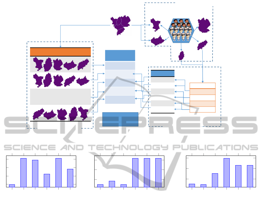
The ﬂow of our experimental study is depicted in Fig-

ure 1. The ﬁgure outlines the three parts of the ex-

perimental design. First, on the left-hand side of the

ﬁgure, the

permutation study

refers to solving the

sub-problems in different order given by all the differ-

ent permutations of the geographical areas. However,

trying all permutations is practical only in small prob-

lems. Therefore, ﬁnding an effective ordering pattern

is the second part of experiment,

observation step

the ﬁgure. This second part solved each sub-problem

using all available workforce, i.e. ignoring if some

workers were assigned in previous sub-problems. The

third part analysed the results from the observation

step in order to deﬁne some strategies to tackle the

sub-problems. Based on this

strategies study

, some

solving strategies were envisaged. Listed in the ﬁgure

are these ordering strategies: Asc-task, Desc-task, Asc-

w&u, etc. More details about these ordering strategies

are provided when decribing the

Observation step

below. Finally, the solutions produced with the differ-

ent ordering strategies are compared to the solutions

produced by the permutation study to evaluate the per-

formance of these ordering strategies.

Permutation Study.

Since the number of permu-

tations grows exponentially with the number of geo-

graphical areas, we performed the permutation study

using only the instances with

|A| = 3

and

|A| = 4

ge-

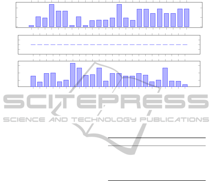
ographical areas. Figure 2 shows the relative gap ob-

tained for the small instances that have 3 regions. Each

sub-ﬁgure shows the results for one instance when

solved using the different permutation orders of the 3

regions. Each bar shows the relative gap between the

solution by the decomposition method and the overall

optimal solution. The ﬁgure shows that the quality

of the obtained solutions for the different permuta-

tions ﬂuctuates considerably. Closer inspection reveals

that in these instances the geographical areas are very

close to each other and sometimes there is an over-

lap between them. The result also reveals that some

permutations clearly give better results. For example,

permutation “1-2-3” for instance WSRP-A-04, permu-

tations “1-2-3” and “2-1-3” for instance WSRP-A-05

and permutations “1-2-3” and “1-3-2” for instance

ICORES2015-InternationalConferenceonOperationsResearchandEnterpriseSystems

288

PERMUTATION ORDER

…

INFORMATION

# task

# worker

# un-assignment

Task : worker

Objective

value

𝒇(𝒙)

𝑓(𝑃𝐸𝑅𝑀1)

𝑓(𝑃𝐸𝑅𝑀2)

𝑓(𝑃𝐸𝑅𝑀3)

…

𝑓(𝑃𝐸𝑅𝑀𝑛)

Split by area

Solve individual sub-problem

using all workers

Get information

Define strategies

Solve in sequence

defined by strategy

Solve sequence

Generate all possible solving orders

Locate strategies

solution on

permutation study

Observation step

Strategies study

Permutation study

STRATEGIES

Asc-task

Desc-task

Asc-w&u

Desc-w&u

Asc-ratio

Desc-ratio

Figure 1: Outline of the experimental study in three parts: permutation study, observation step and strategies study.

1-2-3

1-3-2

2-1-3

2-3-1

3-1-2

3-2-1

Relative gap (%)

WSRP-A-04

1-2-3

1-3-2

2-1-3

2-3-1

3-1-2

3-2-1

WSRP-A-05

1-2-3

1-3-2

2-1-3

2-3-1

3-1-2

3-2-1

WSRP-A-07

Figure 2: Relative gap obtained from solving the 3 instances (WSRP-A-04, WSRP-A-05 and WSRP-A-07) with

|A| = 3

using

the different permutation orders. Each graph shows results for one instance. The bars represent the relative gap between the

solution obtained with the decomposition method and the overall optimal solution.

WSRP-A-07.

Figure 3 shows the relative gap obtained for the

small instances that have 4 regions. Each sub-ﬁgure

shows the result for one instance when solved using

the permutation orders of the 4 regions. Each bar

shows the relative gap between the solution by the de-

composition method and the overall optimal solution.

The ﬁgure reveals an interesting result from instance

WSRP-B-02. The optimal solution value is obtained

for every permutation. Closer inspection reveals that

the decomposition method works very well on this

instance because its geographical areas are well sep-

arated from each other. Therefore, the sub-problem

solutions are part of the complete overall solution and

not many worker assignment conﬂicts arise when solv-

ing the sub-problems. For the other instances, WSRP-

A-02 and WSRP-B-04, the quality of the obtained

solutions ﬂuctuates in the same way as in Figure 2. Re-

sults in Figure 3 indicate that some solutions obtained

with the decomposition approach using some permu-

tations have a considerable gap in quality compared

to the overall optimal solution. The ﬁgure also shows

that some permutations clearly give better results than

others. For example, permutation “1-2-3-4”, “2-1-3-4”

and “2-3-1-4” for instance WSRP-A-02 and permuta-

tion “4-3-2-1” for instance WSRP-B-04.

The conclusion from this permutation study is that

the order in which the sub-problems are solved matters

differently according to the problem instance. More

importantly, the results conﬁrm our assumption that

some particular permutation could produce a very

good result in the decomposition approach. Hence,

the next part of the study is to ﬁnd a good solving

order.

Observation Step

. Here we solve each of the sub-

problems using all available workers and collect the

following values from the obtained solutions: number

of tasks in the sub-problem (# task), minimum number

of workers required in the solution (# min worker),

number of unassigned tasks in the solution (# unas-

MixedIntegerProgrammingwithDecompositiontoSolveaWorkforceSchedulingandRoutingProblem

289

Relative gap (%)

WSRP-A-02

−0.5

0.5

Relative gap (%)

WSRP-B-02

1-2-3-4

1-2-4-3

1-3-2-4

1-3-4-2

1-4-2-3

1-4-3-2

2-1-3-4

2-1-4-3

2-3-1-4

2-3-4-1

2-4-1-3

2-4-3-1

3-1-2-4

3-1-4-2

3-2-1-4

3-2-4-1

3-4-1-2

3-4-2-1

4-1-2-3

4-1-3-2

4-2-1-3

4-2-3-1

4-3-1-2

4-3-2-1

Relative gap (%)

WSRP-B-04

Figure 3: Relative gap obtained from solving the 3 instances (WSRP-A-02, WSRP-B-02 and WSRP-B-04) with

|A| = 4

using

the different permutation orders. Each graph shows results for one instance. The bars represent the relative gap between the

solution obtained with the decomposition method and the overall optimal solution.

signed task) and the ratio of tasks to worker in the solu-

tion (task/worker ratio). Then, we deﬁned six ordering

strategies as follows. Increasing number of tasks in the

sub-problem (Asc-task); decreasing number of tasks

in the sub-problem (Desc-task); increasing sum of

minimum workers required and unassigned tasks (Asc-

w&u); decreasing sum of minimum workers required

and unassigned tasks (Desc-w&u); increasing ratio

of tasks to worker (Asc-ratio) and decreasing ratio of

tasks to worker (Desc-ratio).

Strategies Study

. The GDCA approach is again

executed using the 6 ordering strategies listed above

to tackle the sub-problems in each problem instance.

The results are presented in Figure 4 which shows the

relative gap for the 14 small instances in the WSRP-A

and WSRP-B groups. Note that each bar represents

the relative gap obtained with each strategy.

From Figure 4, the decomposition technique with

ordering strategies gives solutions with relative gaps

below 50%. On average, the decomposition technique

produces relative gap at 16.36%. Moreover, we can

see that some of the ordering strategies are more likely

to produce better solutions than others. The best per-

forming ordering strategy is Asc-w&u that gives 9

best solutions considering all 14 small instances. The

average gap for the ordering strategies Asc-task, Desc-

task, Asc-w&u, Desc-w&u, Asc-ratio and Desc-ratio

are 14.09%, 19.94%, 11.19%, 19.66%, 15.01% and

18.28% respectively. Table 3 shows a comparison of

relative gap between the best permutation order (see

Permutation study

) and the best ordering strategy. It

Table 3: Relative gap (%) of best permutation VS. best

strategy.

Instance Best permutation Best strategy

WSRP-A-04 3.9 6.4

WSRP-A-05 24.67 24.67

WSRP-A-07 14.43 15.03

WSRP-A-02 2.31 2.32

WSRP-B-02 0 0

WSRP-B-04 7.02 8.86

is clearly shown that solutions from the best ordering

strategy are not much different from the best permu-

tation solution (maximum of 2.5% different). In addi-

tion, two out of six solutions (instance WSRP-A-05

and WSRP-B-02) of the best ordering strategy match

the solution from the best permutation. This shows

that the ordering strategies are able to work well in

other problem instances.

The decomposition method is also able to ﬁnd so-

lutions for the large instances whilst solving those

problems as a whole is not practical in terms of com-

putation time. The results from using the decompo-

sition technique with the 6 ordering strategies on the

large instances are presented in Table 4. The table

shows the objective values of the obtained solutions

as relative gaps cannot be computed because the opti-

mal solutions are not known. The values in

bold

are

the lowest cost (best objective value) obtained among

the six strategies. The table shows that as a whole,

the Desc-ratio and Asc-w&u give four and three best

ICORES2015-InternationalConferenceonOperationsResearchandEnterpriseSystems

290

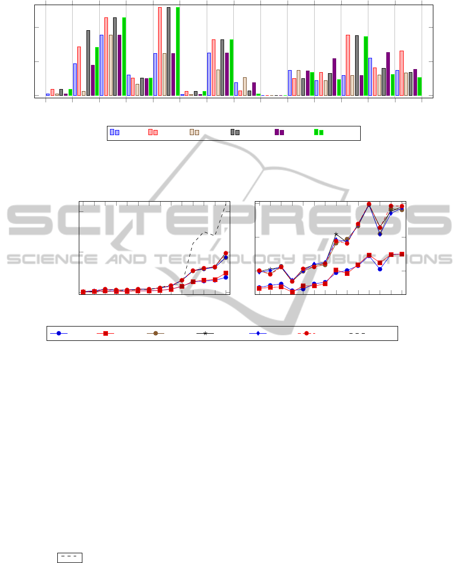
A-01 A-02 A-03 A-04 A-05 A-06 A-07 B-01 B-02 B-03 B-04 B-05 B-06 B-07

WSRP-

Relative gap (%)

Asc-task Desc-task Asc-w&u Desc-w&u Asc-ratio Desc-ratio

Figure 4: Relative gap obtained from solving the 14 small instances using the 6 ordering strategies. Each bar for an instance

represents the relative gap between a solution by the decomposition method using an ordering strategy and the overall optimal

solution.

103

100

200

Problem size (items)

Computation time (seconds)

Small instances

620

647

694

711

759

784

2012

2016

2237

2365

2377

2482

2737

0.5

1.5

·10

Problem size (items)

Large instances

Asc-task Desc-task Asc-w&u Desc-w&u Asc-ratio Desc-ratio Optimal

Figure 5: Computation time (seconds) used in solving small and large instances. Each sub-ﬁgure corresponds to a problem

size category (small and large). The problem size (items) is the summation of #workers and #tasks. Each graph presents the

computation time used by the decomposition method with the different ordering strategies (line with markers) and the time

used for producing the overall optimal solution (dashed line) when possible.

solutions respectively while the others give two best

solutions. On average, the Desc-task strategy gives the

lowest cost solution, around 5.7% less than the highest

average cost strategy (Asc-ratio).

Figure 5 shows, according to the problem size,

the computation times used by the decomposition ap-

proach using the different ordering strategies and the

time used to ﬁnd the overall optimal solution. Each

sub-ﬁgure presents the problem instances classiﬁed

by their size (number of items is

|T | + |C|

). Each

line represents the time used by the ordering strat-

egy in solving the group of 14 problem instances. As

noted before, the time to ﬁnd the optimal solution

represented by is available only for the small

instances. For the smaller instances with less than 89

items, the computation time used by the decomposi-

tion method is not much different from the time used

to ﬁnd the optimal solution. The computation time

used to ﬁnd the optimal solution grows signiﬁcantly

for instances with 89 items and above. For the large in-

stances, it is shown that the computation time used by

the decomposition method goes above 4 hours (14,895

seconds). Also, for the large instances the computa-

tion time used by the ordering strategies Asc-task and

Desc-task is signiﬁcantly less than for the other order-

ing strategies. This is because these ordering strategies

do not require an additional process to retrieve infor-

mation about the problem. Hence, considering both

solution quality and computation time, it can be con-

cluded that Asc-task and Desc-task (best known on

average) should be selected for large instances because

they produce solutions which are not much different

from the other strategies but requiring signiﬁcantly

less computational time (48.3% less on average).

5 CONCLUSION AND FUTURE

WORK

A tailored mixed integer programming model for real-

world instances of a workforce scheduling and routing

MixedIntegerProgrammingwithDecompositiontoSolveaWorkforceSchedulingandRoutingProblem

291

Table 4: Objective value obtained from solving large instances using six ordering strategies.

Instance Asc-task Desc-task Asc-w&u Desc-w&u Asc-ratio Desc-ratio

WSRP-D-01 118,647.95 109,634.79 120,538.27 107,264.93 112,695.33 109,693.81

WSRP-D-02 119,505.44 120,707.43 117,169.05 119,317.34 113,367.92 115,790.07

WSRP-D-03 95,302.20 93,097.74 95,302.20 92,349.70 95,302.20 89,468.63

WSRP-D-04 103,685.14 101,861.74 250,740.31 135,675.84 105,268.17 143,621.85

WSRP-D-05 86,581.13 84,505.24 84,366.48 87,588.51 86,581.13 84,505.24

WSRP-D-06 76,681.66 77,279.43 74,438.87 80,083.86 76,737.43 73,202.04

WSRP-D-07 71,029.11 77,381.16 71,485.90 117,757.75 71,029.11 73,055.89

WSRP-F-01 584,285.07 568,346.64 584,908.75 554,471.47 585,321.17 559,036.26

WSRP-F-02 592,505.48 582,181.95 575,441.87 597,279.38 605,906.81 559,198.12

WSRP-F-03 590,040.74 593,763.31 590,619.01 582,329.81 603,655.07 581,596.60

WSRP-F-04 825,931.68 900,387.30 876,679.55 872,606.58 838,692.36 849,852.84

WSRP-F-05 567,245.71 614,704.32 542,364.31 583,121.68 563,245.40 551,663.99

WSRP-F-06 931,935.20 718,310.26 792,308.91 943,102.96 101,4421.53 777,265.11

WSRP-F-07 696,718.60 777,163.34 684,083.36 777,903.33 874,069.14 875,234.10

Average 390,006.79 387,094.62 390,031.92 403,632.37 410,449.48 388,798.90

Bold text refers to the best solution.

problem is presented. The model is constructed by

incorporating various constraint formulations from the

literature while also adding working region constraints

to the formulation. It is usually the case that models in

the literature for this type of problem are presented but

their solution is approached using alternative methods

such as heuristics because solving the model using

mathematical exact solvers is computationally chal-

lenging. A geographical decomposition with conﬂict

avoidance approach is proposed here to tackle work-

force scheduling and routing problems while still har-

nessing the power of exact solvers. The proposed

decomposition method allows to tackle real-world size

problems for which ﬁnding the overall optimal solu-

tion requires too much computation time. However,

the solution quality ﬂuctuates when changing the order

to tackle the sub-problems deﬁned by the geographi-

cal regions. Exploring all permutation orders to ﬁnd

the one producing the best results is not practical for

larger problems (e.g. more than 6 geographical ar-

eas). In this work, six ordering strategies are proposed

for obtaining high-quality solutions within acceptable

computation time. Our future research will explore

ways to replace the originally deﬁned geographical

areas with automated clustering to deﬁne well sepa-

rated geographical areas even in cases where the areas

deﬁned by the problem data are not well separated.

ACKNOWLEDGEMENTS

Special thanks to the Development and Promotion for

Science and Technology talents project (DPST, Thai-

land) who providing partial ﬁnancial support. Also, we

are grateful for access to the University of Nottingham

High Performance Computing Facility.

REFERENCES

Akjiratikarl, C., Yenradee, P., and Drake, P. R. (2007). PSO-

based algorithm for home care worker scheduling in the

UK. Computers & Industrial Engineering, 53(4):559–

583, doi:10.1016/j.cie.2007.06.002.

Angelis, V. D. (1998). Planning home assistance for AIDS

patients in the City of Rome , Italy. Interfaces, 28:75–

83.

Barrera, D., Nubia, V., and Ciro-Alberto, A. (2012). A

network-based approach to the multi-activity combined

timetabling and crew scheduling problem: Workforce

scheduling for public health policy implementation.

Computers & Industrial Engineering, 63(4):802–812,

doi:10.1016/j.cie.2012.05.002.

Benders, J. (1962). Partitioning procedures for solving

mixed-variables programming problems. Numerische

Mathematik, 4(1):238–252, doi:10.1007/BF01386316.

Bertels, S. and Torsten, F. (2006). A hybrid setup for a hybrid

scenario: Combining heuristics for the home health

care problem. Computers & Operations Research,

33(10):2866–2890.

Borsani, V., Andrea, M., Giacomo, B., and Francesco, S.

(2006). A home care scheduling model for human re-

sources. 2006 International Conference on Service

Systems and Service Management, pages 449–454,

doi:10.1109/ICSSSM.2006.320504.

Bredstrom, D. and Ronnqvist, M. (2007). A branch and

price algorithm for the combined vehicle routing and

scheduling problem with synchronization constraints.

NHH Dept. of Finance & Management Science Discus-

sion Paper No. 2007/7, (February).

Bredstrom, D. and Ronnqvist, M. (2008). Combined vehi-

cle routing and scheduling with temporal precedence

ICORES2015-InternationalConferenceonOperationsResearchandEnterpriseSystems

292

and synchronization constraints. European Journal of

Operational Research, 191(1):19 – 31.

Castillo-Salazar, J., Landa-Silva, D., and Qu, R. (2014).

Workforce scheduling and routing problems: literature

survey and computational study. Annals of Operations

Research, doi:10.1007/s10479-014-1687-2.

Castro-Gutierrez, J., Landa-Silva, D., and Moreno,

P. J. (2011). Nature of real-world multi-objective

vehicle routing with evolutionary algorithms. Sys-

tems, Man, and Cybernetics (SMC), 2011 IEEE

International Conference on, pages 257–264,

doi:10.1109/ICSMC.2011.6083675.

Cordeau, J.-F., Stojkovic, G., Soumis, F., and Desrosiers,

J. (2001). Benders decomposition for simul-

taneous aircraft routing and crew schedul-

ing. Transportation Science, 35(4):375–388,

doi:10.1287/trsc.35.4.375.10432.

Dantzig, G. B. and Ramser, J. H. (1959). The truck dis-

patching problem. Management Science (pre-1986),

6(1).

Dohn, A., Esben, K., and Jens, C. (2009). The man-

power allocation problem with time windows and job-

teaming constraints: A branch-and-price approach.

Computers & Operations Research, 36(4):1145–1157,

doi:10.1016/j.cor.2007.12.011.

Eveborn, P., Ronnqvist, M., Einarsdottir, H., Eklund, M.,

Liden, K., and Almroth, M. (2009). Operations re-

search improves quality and efﬁciency in home care.

Interfaces, 39(1):18–34, doi:10.1287/inte.1080.0411.

Feillet, D. (2010). A tutorial on column generation and

branch-and-price for vehicle routing problems. 4OR,

8(4):407–424.

Hart, E., Sim, K., and Urquhart, N. (2014). A real-world em-

ployee scheduling and routing application. In Proceed-

ings of the 2014 Conference Companion on Genetic

and Evolutionary Computation Companion, GECCO

Comp ’14, pages 1239–1242, New York, NY, USA.

ACM.

Kergosien, Y., Lente, C., and Billaut, J.-C. (2009). Home

health care problem, an extended multiple travelling

salesman problem. In Proceedings of the 4th multidis-

ciplinary international scheduling conference: Theory

and applications (MISTA 2009), Dublin, Ireland, pages

85–92.

Landa-Silva, D., Wang, Y., Donovan, P., Kendall, G., and

Way, S. (2011). Hybrid heuristic for multi-carrier trans-

portation plans. In The 9th Metaheuristics Interna-

tional Conference (MIC 2011), pages 221–229.

Liu, R., Xie, X., and Garaix, T. (2014). Hy-

bridization of tabu search with feasible and

infeasible local searches for periodic home

health care logistics. Omega, 47(0):17 – 32,

doi:http://dx.doi.org/10.1016/j.omega.2014.03.003.

Mankowska, D., Meisel, F., and Bierwirth, C. (2014). The

home health care routing and scheduling problem with

interdependent services. Health Care Management

Science, 17(1):15–30, doi:10.1007/s10729-013-9243-

Mercier, A., Cordeau, J.-F., and Soumis, F. (2005). A com-

putational study of Benders decomposition for the in-

tegrated aircraft routing and crew scheduling problem.

Computers & Operations Research, 32(6):1451 – 1476,

doi:http://dx.doi.org/10.1016/j.cor.2003.11.013.

Perl, J. and Daskin, M. S. (1985). A warehouse

location-routing problem. Transportation Re-

search Part B: Methodological, 19(5):381 – 396,

doi:http://dx.doi.org/10.1016/0191-2615(85)90052-9.

Pillac, V., Gueret, C., and Medaglia, A. (2012). On the

dynamic technician routing and scheduling problem.

In Proceedings of the 5th International Workshop

on Freight Transportation and Logistics (ODYSSEUS

2012), page id: 194, Mikonos, Greece.

Ralphs, T. K. and Galati, M. V. (2010). Decomposition

methods for integer programming. Wiley Encyclope-

dia of Operations Research and Management Science,

doi:10.1002/9780470400531.eorms0233.

Rasmussen, M. S., Justesen, T., Dohn, A., and

Larsen, J. (2012). The home care crew schedul-

ing problem: Preference-based visit clustering

and temporal dependencies. European Jour-

nal of Operational Research, 219(3):598–610,

doi:http://dx.doi.org/10.1016/j.ejor.2011.10.048.

Reimann, M., Doerner, K., and Hartl, R. F. (2004). D-Ants:

Savings based ants divide and conquer the vehicle

routing problem. Computers & Operations Research,

31(4):563 – 591, doi:http://dx.doi.org/10.1016/S0305-

0548(03)00014-5.

Trautsamwieser, A. and Hirsch, P. (2011). Optimization of

daily scheduling for home health care services. Journal

of Applied Operational Research, 3:124–136.

Vanderbeck, F. (2000). On Dantzig-Wolfe decomposition in

integer programming and ways to perform branching

in a branch-and-price algorithm. Operations Research,

48(1):111.

Vanderbeck, F. and Wolsey, L. (2010). Reformulation and

decomposition of integer programs. In Junger, M. et al.,

editors, 50 Years of Integer Programming 1958-2008,

pages 431–502. Springer Berlin Heidelberg.

MixedIntegerProgrammingwithDecompositiontoSolveaWorkforceSchedulingandRoutingProblem

293