
Fast Solving of Influence Diagrams for Multiagent Planning on
GPU-enabled Architectures
Fadel Adoe, Yingke Chen and Prashant Doshi
THINC Lab, Department of Computer Science, University of Georgia, Athens, Georgia, U.S.A.
Keywords:
GPU, Multiagent Systems, Planning, Speed Up.
Abstract:
Planning under uncertainty in multiagent settings is highly intractable because of history and plan space com-
plexities. Probabilistic graphical models exploit the structure of the problem domain to mitigate the com-
putational burden. In this paper, we introduce the first parallelization of planning in multiagent settings on
a CPU-GPU heterogeneous system. In particular, we focus on the algorithm for exactly solving interactive
dynamic influence diagrams, which is a recognized graphical models for multiagent planning. Beyond paral-
lelizing the standard Bayesian inference, the computation of decisions’ expected utilities are parallelized. The
GPU-based approach provides significant speedup on two benchmark problems.
1 INTRODUCTION
Planning under uncertainty in multiagent settings is
a very hard problem because it involves reasoning
about the actions and observations of multiple agents
simultaneously. In order to formally study this prob-
lem, the approach is to generalize single-agent plan-
ning frameworks such as the partially observable
Markov decision process (POMDP) (Smallwood and
Sondik, 1973) to multiagent settings. This has led
to the decentralized POMDP (Berstein et al., 2005)
for multiagent planning in cooperative settings and
the interactive POMDP (Gmytrasiewicz and Doshi,
2005) for individual planning in cooperative or non-
cooperative multiagent settings. A measure of the
involved computational complexity is available by
noting that the problem of solving a decentralized
POMDP exactly for a finite number of steps is NEXP
complete (Bernstein et al., 2002).
Some of the complexity of multiagent planning
may be mitigated by exploiting the structure in the
problem domain. Often, the state of the problem can
be factored into random variables and the conditional
independence between the variables may be naturally
exploited by representing the planning problem us-
ing probabilistic graphical models. An example of
such a model is the interactive dynamic influence di-
agram (I-DID) (Doshi et al., 2009) that generalizes
the well-known DID (Howard and Matheson, 1984),
which may be viewed as a graphical counterpart of
POMDP, to multiagents settings in the same way that
an interactivePOMDP generalizes the POMDP. In ad-
dition to modeling the problem structure, graphical
models provide an intuitive language for representing
the planning problem thereby serving as an important
tool to enable multiagent planning.
1
Emerging applications in automated vehicles that
communicate (Luo et al., 2011), integration with the
belief-desire-intention framework (Chen et al., 2013),
and for ad hoc teamwork (Chandrasekaran et al.,
2014) motivate improved solutions of I-DIDs. While
techniques exist for introducing further efficiency into
solving I-DIDs (Zeng and Doshi, 2012), we may
also explore parallelizing its solution algorithm on
new high-performance computing architectures such
as those utilizing graphic processing units (GPU). A
GPU consists of an array of streaming multiproces-
sors (SM) connected to a shared memory. Each SM
typically consists of a set of streaming processors.
Consequently, a GPU supplements the CPU by en-
abling massive parallelization of simple computations
that do not require excessive memory.
Our contribution in this paper is ways of paral-
lelizing multiple steps of the algorithm for exactly
solving I-DIDs on CPU-GPU architectures. This pro-
motes significantly faster planning on benchmark and
large multiagent problems up to an order of magni-
tude in comparison to the run-time performance of the
1
A GUI-based software application called Netus is
freely available from http://tinyurl.com/mwrtlvg for design-
ing I-DIDs.
183
Adoe F., Chen Y. and Doshi P..
Fast Solving of Influence Diagrams for Multiagent Planning on GPU-enabled Architectures.
DOI: 10.5220/0005224001830195
In Proceedings of the International Conference on Agents and Artificial Intelligence (ICAART-2015), pages 183-195
ISBN: 978-989-758-074-1
Copyright
c
2015 SCITEPRESS (Science and Technology Publications, Lda.)

existing algorithm. In addition to the usual chance,
decision and utility nodes, I-DIDs include a new type
of node called the model node and a new link called
the policy link between the model node and a chance
node that represents the distribution over the other
agent’s actions given its model.
The algorithm for solving an I-DID expands a
given two-time slice I-DID over multiple steps and
collapses the I-DID into a flat DID. We may then
use the standard sum-max-sum rule and a general-
ized variable elimination algorithm for IDs (Koller
and Friedman, 2009) to compute the maximum ex-
pected utilities of actions at each decision node to
solve the I-DID. Multiple models in the model node
are recursively solved in an analogous manner. Our
approach is to parallelize two steps of this algorithm:
(i) The four operations involved in the sum-max-
sum rule: max-marginalization (of decisions), sum-
marginalization (of chance variables), factor-product
(of probabilities and utilities) and factor-addition (of
utilities) are parallelized on the GPU. (ii) Probabil-
ity factors in the variable elimination could be large
joints of the Bayesian network at each time slice, and
we parallelize the message passing performed on a
junction tree during the inference, on the GPU.
We evaluate the parallelized I-DID solution algo-
rithm on two benchmark planning domains, and show
more than an order of magnitude in speed up on some
of the problems compared to the previous algorithm.
We evaluate on planning domains that in size of the
state, action and observation spaces, and extend the
planning over longer horizons. In addition, we study
the properties of our algorithm by allocating it in-
creasing concurrency on the GPU and show that it’s
run time improves up to a point beyond which the
gains are lost.
The rest of the paper is organized as follows. Sec-
tion 2 provides preliminaries about the I-DID and
concepts of GPU-based programming. Section 3 re-
views related work. Section 4 proposes a GPU-based
approach to exactly solve the I-DID in parallel. Sec-
tion 6 theoretically analyze the speed up. Section 7
demonstrates the speed up by the proposed approach
on two problems. Section 8 concludes this paper.
2 BACKGROUND
In this section, we briefly review the probabilistic
graphical model, DID, and its generalization to mul-
tiagent settings, I-DID. General principles behind
GPU-based programming are also briefly described.
2.1 Dynamic Influence Diagram
A DID, D, is a directed acyclic graph over a set of
nodes: chance nodes C (ellipses), representing ran-
dom variables; decision nodes D (rectangles), model-
ing the action choices; utility nodes U (diamonds),
representing rewards based on chance and decision
node values, and a set of arcs representing depen-
dencies. Conditional probability distributions, P, and
utility functions, R, are associated with the chance
and utility nodes, respectively. In rest of the paper,
nodes and variables are used interchangeably.
The domain of a variable Q, denoted as dom(Q),
contains its possible values. The parent of Q, de-
noted as Pa
Q
, is a set of variables having direct
arcs incident on Q. The domain of Pa
Q
, dom(Pa
Q
),
is the Cartesian product of the individual domains:
dom(Pa
Q
) =
∏
Z∈Pa
Q
dom(Z), and a value of this do-
main is denoted as, pa
Q
. A probability factor, φ(Q) =
P(Q|Pa
Q
), which defines conditional probability dis-
tribution given instantiation of parent variables, is at-
tached to each chance variable Q ∈ C. We use Ch
Q
to
denote Q’s children. A utility factor, ψ(U) = R(Pa
U
),
where R returns real-valued rewards, is associated
with each utility node, U ∈ U. The variables involved
in a probability or utility factor become the domain of
this factor, for example, dom(φ(Q)) = {Q} ∪ Pa
Q
.
A policy for decision node, D
i
∈ D, is a mapping,
δ
i
: dom(Pa
D
i
) → dom(D
i
), i.e., δ
i
(pa
D
i
) = d
i
. A pol-
icy for the decision problem is a sequence of policies
for all the decision nodes. The solution of a DID is a
strategy that maximizes the expected value MEU(D),
computed using the sum-max-sum rule (Koller and
Friedman, 2009):
∑
I
0
max
D
1
∑
I
1
... max
D
n
∑
I
n
(
∏
Q
i
∈C
P(Q
i
|Pa
Q
i
) ·
∑
C,D
R(C,D))
where I
0
, I
1
, ..., I
n−1
is the set of chance variables in-
cident on the decision nodes, D
1
, D
2
, ..., D
n
, thereby
forming the information sets.
The MEU may be computed by repeatedly elimi-
nating variables. Let Φ and Ψ be the set of probability
and utility factors, respectively. Given variable Q, the
probability and utility factors having Q in their do-
main are denoted as Φ
Q
and Ψ
Q
, respectively. After
Q is eliminated, the factor sets are updated as follows:
Φ = (Φ\ Φ
Q
) ∪ {φ
\Q
} and Ψ = (Ψ \ Ψ
Q
) ∪ {
ψ
\Q
φ
\Q
}.
Here, φ
\Q
=
∑
Q
∏
Φ
Q
and ψ
\Q
=
∑
Q
∏
Φ
Q
(
∑
Ψ
Q
)
when Q is a chance variable; if Q is a deci-
sion variable, then, φ
\Q
= max
Q
∏
Φ
Q
and ψ
\Q
=
max
Q
∏
Φ
Q
(
∑
Ψ
Q
).
ICAART2015-InternationalConferenceonAgentsandArtificialIntelligence
184

2.2 Interactive DID
Interactive DID (I-DID) (Doshi et al., 2009) mod-
els an individual agent’s planning (sequential deci-
sion making) in a multiagent setting. In a I-DID,
other agents’ candidate behaviors are modeled as
they impact the common states and rewards during
the subject agent’s decision-making process. Simul-
taneously, other agents also reason about the sub-
ject agent’s possible actions in their decision making.
This recursive modeling is encoded in an auxiliary
data item called the model node M
t
j,l−1
which con-
tains models of the other agent, say j of level l−1 and
chance node A
j
which represents the distribution over
j’s actions. The link between M
t
j,l−1
and A
t
j
, named as
policy link, indicates that the other agent’s predicted
action is based on its models. The models can be
DIDs, I-DIDs or simply probability distributions over
actions. The link between M
t
j,l−1
and M
t+1
j,l−1
, called
model update link, represents the update of j’s model
over time.
Example 1 (Multiagent tiger problem (Gmy-
trasiewicz and Doshi, 2005)). Consider two agents
standing in front of two closed doors with a tiger or
some gold behind each door. If an agent opens a door
with a tiger behind it, it receives a penalty, otherwise
a reward. Agents can listen for growls to gain in-
formation about the tiger’s location as well as hear
creaks if the other agent opens a door. But, listening
is not accurate. When the agent receives a reward or
penalty, the game is reset. There is another agent j
with the same character sharing the environment with
agent i without noticing the existence of agent i. They
receives reward or penalty together, therefore agent i
needs to take into account agent j’s behavior. A two
time-slice I-DID for agent i situated in the multiagent
tiger problem is depicted in Fig. 1.
TL
t
GC
t
A
i
t
R
i
TL
t+1
GC
t+1
A
i
t+1
R
i
M
j,l-1
t
A
j
t
M
j,l-1
t+1
A
j
t+1
Figure 1: A two time-slice I-DID for agent i in the tiger
problem. Policy links are marked as dash lines, while model
update links are marked as dotted lines. TL stands for ‘Tiger
Location’ and GC stands for ‘Growl&Creak’.
Solving an I-DID (shown in Fig. 3) requires solv-
ing the lower-level models, and this recursive pro-
cedure ends at level 0 where the I-DID reduces to a
DID (Line 4). The policies from solving lower-level
models are used to expand the next higher-level I-DID
(Line 5 - 10). We may then replace the model nodes,
policy and the model update links with regular chance
nodes and dependency links. States of the nodes and
parameters of the links are specified according to the
obtained policies (Line 11 - 13). Subsequently, an I-
DID becomes a regular DID, whose MEU is obtained
(Line 15). Doshi and Zeng (2009) provide more de-
tails about I-DIDs including an algorithm for solving
it optimally.
Example 2. The I-DID shown in Fig. 1 is expanded
as shown in Fig. 2. GC denotes a chance variable
for observations of Growl&Creak, and the remaining
chance nodes are grouped and denoted by X
i
for con-
venience. The MEU is calculated as follows.
MEU[D] =
∑
X
t
i
max
A
t
i
∑
GC
t
P(X
t
i
)P(GC
t
|X
t
i
)
∑
X
t+1
i
max
A
t+1
i
∑
GC
t+1
P(X
t+1
i
|X
t
i
,A
t
i
)P(GC
t+1
|X
t+1
i
)
[R
t
i
(A
t
i
,X
t
i
) + R
t+1
i
(A
t+1
i
,X
t+1
i
)]
(1)
TL
t
GC
t
A
i
t
R
i
TL
t+1
GC
t+1
A
i
t+1
R
i
A
j
t
A
j
t+1
A
j
2
A
j
1
Mod[M
j
t
]
O
j
t+1
O
j
1
O
j
2
A
j
2
A
j
1
Mod[M
j
t+1
]
A
j
3
A
j
4
X
i
t
X
i
t+1
Figure 2: The flat two time-slice DIDs for the tiger problem.
Model nodes are replaced by a set of ordinary chance nodes.
All hidden variables are grouped as X
i
.
2.3 GPU and CUDA
Graphics processing units (GPUs) were originally de-
signed for rendering computer graphics.
In a GPU, there are a number of streaming multi-
processsors (SM), each containing a set of stream pro-
cessors, registers and shared local memory (SMEM).
At run time, a set of parallelized computation tasks re-
ferred to as a thread block are executed on a SM and
distributed across the processors. In order to achieve
good performance, it is crucial to map algorithms to
the GPU architecture efficiently, which is optimized
for high throughput. For example, designs that favor
coalesced memory access are cost-effective. In the
past decade, general purpose computing on the GPU
has increased with a focus on bridging the gap be-
tween GPUs and CPUs by letting GPUs handle the
FastSolvingofInfluenceDiagramsforMultiagentPlanningonGPU-enabledArchitectures
185

I-DID EXACT
(level l ≥ 1 I-DID or level 0 DID, horizon T)
Expansion Phase
1. For t from 0 to T − 1 do
2. If l ≥ 1 then
Populate M
t+1
j,l−1
3. For each m
t
j
in Range(M
t
j,l−1
) do
4. Recursively call algorithm with the l − 1
I-DID (or DID) that represents m
t
j
and
the horizon, T − t
5. Map the decision node of the solved I-DID
(or DID), OPT(m
t
j
), to the corresponding
chance node A
j
6. For each a
j
in OPT(m
t
j
) do
7. For each o
j
in O
j
(part of m
t
j
) do
8. Update j’s belief,
b
t+1
j
← SE(b
t
j
,a
j
,o
j
)
9. m
t+1
j
← New I-DID (or DID) with
b
t+1
j
as the initial belief
10. Range(M
t+1
j,l−1
)
∪
← {m
t+1
j
}
11. Add the model node, M
t+1
j,l−1
, and the model update
link between M
t
j,l−1
and M
t+1
j,l−1
12. Add the chance, decision, and utility nodes for t + 1
time slice and the dependency links between them
13. Establish the CPDs for each node
Solution Phase
14. If l ≥ 1 then
15. Represent the model nodes, policy links and the
model update links as in Fig. 1 to obtain the DID
16. Apply the standard sum-max-sum rule to solve the
expanded DID (other solution approaches may also be used)
Figure 3: Algorithm for exactly solving a level l ≥ 1 I-DID
or level 0 DID expanded over T time steps.
most intensive computing while still leaving control-
ling tasks to CPU. CUDA provided by NVIDIA is
a general-purpose parallel computing programming
model for NVIDIA’s GPUs. CUDA abstracts most
operational details of GPU and alleviates the devel-
oper from the technical burden GPU-oriented pro-
gramming. An important component of a CUDA pro-
gram is a kernel, which is a function that executes in
parallel on a thread block.
3 RELATED WORK
Multiple frameworks formalize planning under un-
certainty in settings shared with other agents who
may have similar or conflicting objectives. A rec-
ognized framework in this regard is the interactive
POMDP (Gmytrasiewicz and Doshi, 2005) that fa-
cilitates the study of planning in partially observ-
able multiagent settings where other agents may
be cooperative or non-cooperative. I-DIDs (Doshi
et al., 2009) are a graphical counterpart of interactive
POMDPs and have the advantage of a representation
that explicates the embedded domain structure by de-
composing the state space into variables and relation-
ships between the variables.
I-DIDs contribute to a promising line of research
on graphical models for multiagent decision making
and planning, which includes multiagent influence di-
agrams (MAID) (Koller and Milch, 2001), networks
of influence diagrams (NID) (Gal and Pfeffer, 2008),
and limited memory influence diagram based play-
ers (Søndberg-Jeppesen et al., 2013). I-DIDs differ
from MAIDs and NIDs by offering a subjective per-
spective to the interaction and solutions not limited
to equilibria, by ascribing other agents with a distri-
bution of non-equilibrium behaviors as well. Impor-
tantly, I-DIDs offer solutions over extended time in-
teractions, where agents act and update their beliefs
over others’ models which are themselves dynamic.
Previous uses of CPU-GPU heterogeneous sys-
tems in the context of graphical models focus on
speeding up exact inference in Bayesian networks due
to parallelization (V. Kozlov and Pal Singh, 1994;
Jeon et al., 2010; Xia and Prasanna, 2008). For ex-
ample, Jeon et al. (2010) report speedup factors in the
range from 5 to 12 for both marginal and most proba-
ble inference in junction trees. In comparison, we el-
evate the problem from performing inference in junc-
tion trees to finding optimal policies in I-DIDs and
DIDs. As solving I-DIDs requires performing infer-
ence on the underlying Bayesian network in each time
slice, our approach also parallelizes exact inference
using junction trees in a manner similar to previous
work (Zheng et al., 2011). Additionally, we provide a
fast method for evaluating the sum-max-sum rule for
DIDs by parallelizing component operations such as
sum-marginalization and others on a GPU.
4 PARALLELIZED I-DID EXACT
FOR CPU-GPU SYSTEMS
Our approach revises the algorithm, I-DID Exact, pre-
sented in Fig. 3 by parallelizing two component steps
for utilization on a CPU-GPU heterogeneous comput-
ing architecture and through leveraging some of the
recent advances in parallelizing inference in Bayesian
networks.
4.1 Parallelizing Sum-Max-Sum Rule
for MEU
A solution of the sum-max-sum rule mentioned in
Section 2 gives the maximum expected utility of the
ICAART2015-InternationalConferenceonAgentsandArtificialIntelligence
186

flat DID that results from transforming the I-DID. The
temporal structure of the DID provides an ordering of
the chance, decision and utility variables that is uti-
lized by generalized variable elimination for IDs to
compute the MEU. In our two-time slice DID for the
multiagent tiger problem, the elimination ordering is:
X
t+1
, Y
t+1
, A
t+1
i
, X
t
, Y
t
, A
t
i
, where X and Y are the
sets of hidden variables and those in the information
set of a decision variable in each time slice, respec-
tively. The sum-max-sum rule does not specify an
ordering between the variables X and Y.
4.1.1 Memory-efficient Variable Elimination for
DIDs
In order to efficiently use the CPU-GPU memory, we
design the variable elimination memory efficiently.
Specifically, instead of keeping the entire DID in
memory while performing variable elimination, we
lazily bring the minimal set of the other variables and
their factors that are needed in order to eliminate the
variable in question. We refer to this set of variables
as a cover set. We first revisit the definition of a
Markov blanket of a variable.
Definition 1 (Markov blanket, Pearl (1998)). The
Markov blanket of a random variable Q, denoted as
MB(Q), is the minimal set of variables that makes Q
conditionally independent of all other variables given
MB(Q). Formally, Q is conditionally independent of
all other variables in the network given its parents,
children, and children’s parents.
Definition 2 (Cover set). The cover set of a random
variable, Q, denoted by CS(Q) is defined as:
CS(Q) = {Q} ∪ MB(Q).
Notice that the cover set of Q consists of itself
and its Markov blanket. Furthermore, we make the
following straightforward observation:
Observation 1. CS(Q) is exactly identical to the
union of the domains of the factor of Q and the factors
of the children of Q,
CS(Q) = dom(φ
Q
)
[
Z∈Ch
Q
dom(φ
Z
)
Let X be the set of variables in the elimination or-
der that precedes Q. As the cover sets of variables in
X would be in memory already, we define an incre-
mental cover set below that is the set of all variables
in the cover set less all those variables contained in the
cover sets of the variables preceding Q in the elimina-
tion ordering.
Definition 3 (Incrementalcoverset). The incremental
cover set of a random variable, Q, denoted by ICS(Q)
is defined as:
ICS(Q) = {Q} ∪ MB(Q) \
[
X∈X
CS(X),
where X are the variables that preceded Q in the
elimination ordering.
Factors related to variables in ICS(Q) need to be
additionally fetched into memory because the latter
cover sets are already in memory and overlapping
variables need not be fetched. Lemma 1 provides a
simple way to determine the incremental cover set.
Lemma 1. As variable elimination proceeds, let F
Q
be the set of all factors not previously loaded in mem-
ory with Q in each of their domains. Then, the union
of all variables in the domains of F
Q
, denoted as ∆
Q
forms the incremental cover set of Q.
Proof. For the base case, let Q be the first variable
to be eliminated. The union of domains of all fac-
tors with Q in their domains is: ∆
Q
= dom(φ
1
(X
1
)) ∪
dom(φ
2
(X
2
)) ∪ . ..dom(φ
n
(X
n
)). We will show that
∀y ∈ X
i
, y ∈ MB(Q) or y = Q for i ∈ [1, n]. Suppose
that ∃y ∈ X
i
and y /∈ MB(Q) and y 6= Q. Given the
definition of the Markov blanket, y is not a child of Q
or parent of a child of Q. Therefore, from Observa-
tion 1, the corresponding factor, φ
i
, cannot contain Q
in its domain. This is a contradiction and no such y
exists. Therefore, ∀y ∈ X
i
, y ∈ MB(Q) or y is Q.
Let Q
k
be the k
th
variable to be eliminated. As
the inductive hypothesis, ∆
Q
k
= {Q
k
} ∪ MB(Q
k
) \
S
X∈X
CS(X). For the inductive step, let Q
k+1
be the
next variable to be eliminated. Notice that
∆
Q
k
= ∆
Q
k+1
∪CS(Q
k
) ∪ dom(Φ
Q
k
\Q
k+1
) \ dom(Φ
Q
k+1
\Q
k
)
where Φ
Q
k
\Q
k+1
are the factors with Q
k
in their do-
mains and not Q
k+1
– these would be absent from
∆
Q
k+1
– and Φ
Q
k+1
\Q
k
are the factors with Q
k+1
and
not Q
k
in their domains.
We may rewrite the above as:
∆
Q
k+1
= ∆
Q
k
∪ dom(Φ
Q
k+1
\Q
k
) \ dom(Φ
Q
k
\Q
k+1
) \CS(Q
k
)
= dom(Φ
Q
k+1
\Q
k
) ∪ ∆
Q
k
\ dom(Φ
Q
k
\Q
k+1
) \CS(Q
k
)
As ∆
Q
k
denotes the domains of all factors with Q
k
and additionally, with Q
k+1
being present or absent,
∆
Q
k
= dom(Φ
Q
k
,Q
k+1
) ∪ dom(Φ
Q
k
\Q
k+1
) \
S
X∈X
CS(X).
Using this in the above equation,
∆
Q
k+1
= dom(Φ
Q
k+1
\Q
k
) ∪ dom(Φ
Q
k
,Q
k+1
)
∪dom(Φ
Q
k
\Q
k+1
) \ dom(Φ
Q
k
\Q
k+1
)
\
S
X∈X
CS(X)\CS(Q
k
)
= dom(Φ
Q
k+1
\Q
k
) ∪ dom(Φ
Q
k
,Q
k+1
)
\
S
X∈X
CS(X)\CS(Q
k
)
= dom(Φ
Q
k+1
) \
S
X∈X∪Q
k
CS(X)
We may apply a proof similar to that in the base
case to the first term above. Therefore,
∆
Q
k+1
= {Q
k+1
} ∪ MB(Q
k+1
) \
S
X∈X∪Q
k
CS(X)
= ICS(Q
k+1
)
FastSolvingofInfluenceDiagramsforMultiagentPlanningonGPU-enabledArchitectures
187

Next, we establish the benefits and correctness of
solely considering the cover set of Q in Theorem 1.
We define the joint probability distribution of the vari-
ables in the cover set first.
Definition 4 (Factored joint probability distribution of
cover set). The factored joint probability distribution
for a cover set of a random variable, Q, is defined as:
P(Q|Pa
Q
)
∏
Z∈Ch
Q
P(Z|Pa
Z
)
Theorem 1. Let Φ
Q
(Ψ
Q
) be a set of relevant proba-
bility (or utility) factors required to compute the new
factor φ
Q
(ψ
Q
) for eliminating variable Q. All the
variables in the domain of Φ
Q
(Ψ
Q
) exactly comprise
the cover set of Q, CS(Q).
Proof. The set of relevant probability factors Φ
Q
can be separated into two categories: P(Q|Pa
Q
) and
P(X|Pa
X
) where X ∈ Ch
Q
. Consequently, the vari-
able in domains of factors in Φ
Q
are included in
Pa
Q
∪Ch
Q
S
Z∈Ch
Q
Pa
Z
∪ {Q}, which is the cover set
of Q by definition.
Assume there exists a variable Y 6= Q, Y ∈
CS(Q) and Y does not appear in either P(Q|Pa
Q
) or
P(X|Pa
X
) where X ∈ Ch
Q
. In other words, Y /∈ Pa
Q
,
Y /∈ Ch
Q
and Y /∈
S
Z∈Ch
Q
Pa
Z
. Consequently, Y /∈
MB(Q). As Y 6= Q, therefore Y /∈ CS(Q), but this
is a contradiction. Therefore, all variables in CS(Q)
appear in the relevant factors. A similar argument is
applicable to the utility factors Ψ
Q
.
Thus, the cover set of a variable, Q, locally iden-
tifies those variables whose factors change on elimi-
nating Q. These factors contain Q in their domains.
The alternative is a naive global method that searches
over all factors and identifies those with Q in their do-
mains. We illustrate the use of the cover set in elimi-
nating chance and decision variables in the context of
the multiagent tiger problem below.
Example 3 (Variable elimination using cover set).
The two-time slice flat DID is shown in Fig. 4(a). For
clarity, the hidden chance variables in each time slice
are replaced with X
i
thereby compactingthe DID. The
MEU for the DID is given by Equation 1. The tempo-
ral structure of the DID induces a partial ordering for
the elimination of the variables in the rule above. In
the context of Fig. 4(a), this ordering is: X
t+1
i
, A
t+1
i
,
GC
t+1
, X
t
i
, A
t
i
, GC
t
.
We begin by eliminating X
t+1
i
from the DID. Theo-
rem 1 allows us to focus on the cover set of X
t+1
i
only,
which is shown in Fig. 4(b).
A
i
t
GC
t
GC
t+1
X
i
t
X
i
t+1
A
i
t+1
R
i
t
R
i
t+1
A
i
t
GC
t
GC
GC
t
+
1
X
i
t
X
i
t
+
1
A
i
t
+
1
R
i
R
R
i
R
R
(a)
A
i
t
GC
t
GC
t+1
X
i
t
X
i
t+1
A
i
t+1
R
i
t
R
i
t+1
(d)
A
i
t
GC
t
GC
t+1
X
i
t
R
i
t
R
i
t+1
(b)
GC
t
(c)
A
i
t
GC
t+1
X
i
t
A
i
t+1
R
i
t
R
i
t+1
A
i
t
+
1
(e)
A
i
t
GC
t
X
i
t
R
i
t
R
i
t+1
(f)
A
i
t
GC
t
R
i
t
R
i
t+1
Figure 4: An illustration of variable elimination for DIDs.
The incremental cover set for each variable is marked using
a dashed line. In (a− f), the DID is progressively reduced
following the elimination order: {X
t+1
i
,A
t+1
i
,GC
t+1
,X
t
i
}.
CS(X
t+1
i
) ← {X
t+1
i
}
[
MB(X
t+1
i
)}
← {X
t+1
i
,GC
t+1
,X
t
i
,A
t
i
}
ψ
1
(GC
t+1
,X
t
i
,A
t
i
,A
t+1
i
) =
∑
X
t+1
i
P(CS(X
t+1
i
)) R
t+1
i
(A
t+1
i
,X
t+1
i
)
=
∑
X
t+1
i
P(X
t+1
i
,GC
t+1
|X
t
i
,A
t
i
) × R
t+1
i
(A
t+1
i
,X
t+1
i
)
Decision variable, A
t
i
, in the probability factor is
converted into a random variable with a uniform dis-
tribution over its states. We update the set of all utility
factors as: Ψ ← {ψ
1
(GC
t+1
,X
t
i
,A
t
i
,A
t+1
i
)}
Next, we eliminate A
t+1
i
from the reduced DID.
Figure 4(c) shows the incremental cover set of A
t+1
i
with the dashed loop: A
t+1
i
and its factors addition-
ally need to be fetched into memory.
CS(A
t+1
i
) ← {A
t+1
i
,GC
t+1
,A
t
i
}
ψ
2
(GC
t+1
,X
t
i
,A
t
i
) = max
A
t+1
i
ψ
1
(GC
t+1
,X
t
i
,A
t
i
,A
t+1
i
)
The set of utility factors updates to Ψ ←
{ψ
2
(GC
t+1
,X
t
i
,A
t
i
)}.
The DID reduces to the one shown in Fig. 4(d),
from which we now eliminate GC
t+1
. The incremental
cover set of this variable is empty as all the variables
in its cover set were utilized previously and preexist in
memory.
ICAART2015-InternationalConferenceonAgentsandArtificialIntelligence
188

CS(GC
t+1
) ← {GC
t+1
,A
t
i
}
ψ
3
(X
t
i
,A
t
i
) =
∑
GC
t+1
P(GC
t+1
|A
t
i
) ψ
2
(GC
t+1
,X
t
i
,A
t
i
)
The set of utility factors now becomes: Ψ ←
{ψ
3
(X
t
i
,A
t
i
)}.
Finally, we eliminate X
t
i
and GC
t
after fetching
GC
t
(and its factors) into memory.
CS(X
t
i
) ← {X
t
i
,GC
t
}
ψ
4
(A
t
i
,GC
t
) =
∑
X
t
i
P(GC
t
|X
t
i
)
R
t
i
(X
t
i
,A
t
i
) + ψ
3
(X
t
i
,A
t
i
)
The utility factor set becomes Ψ ←
{ψ
4
(A
t
i
,GC
t
)}.
Maximizing over A
t
i
and sum marginalization of
GC
t
will yield an empty factor set and the decision
that maximizes the expected utility of the DID.
4.1.2 Speeding Up Factor Operations using GPU
We perform the product operation between probabil-
ity and utility factors in parallel on a GPU. The oper-
ation is a pointwise product of the entries in factors.
When there are common variables, only entries with
the same value of the common variables is multiplied.
For convenience, we denote R
t
i
(X
t
i
,A
t
i
) + ψ
3
(X
t
i
,A
t
i
)
simply as ψ
′
3
(X
t
i
,A
t
i
).
In order to parallelize the factor product, indices
of entries to be multiplied in the factors are needed.
Previous parallelization of inference in Bayesian net-
works sought to minimize the size of the index map-
ping table for GPUs (Jeon et al., 2010) due to the SM
memory limitation. The entire mapping table was de-
composed into smaller ones each giving the mapped
indices of the entries in the second factor for each
non-common variable in the first factor. Our utility
factor product follows the similar principle of mes-
sage passing for belief propagation in junction trees.
Pr(X
i
t
,GC
t
)
Tag
a
0
b
0
c
0
gc
0
a
1
b
0
c
0
gc
0
a
0
b
1
c
0
gc
0
...
a
0
b
0
c
0
gc
1
...
a
1
b
1
c
1
gc
1
000
100
010
111
000
...
...
ψ’
3
(X
i
t
,A
i
t
)
Tag
a
0
b
0
c
0
a
0
a
0
b
0
c
0
a
0
a
0
b
0
c
0
a
0
...
a
0
b
0
c
1
a
1
...
a
1
b
1
c
1
a
1
000
100
010
111
001
...
...
SMEM
SMEM
Spawn |Pr(X
i
t
,GC
t
)|
threads
1
st
iter
N
th
iter
a
0
b
0
c
0
a
1
000
...
Figure 5: The index mapping table. We assume that all
variables are boolean. SMEM denotes shared memory.
Entries in a factor are indexed according to
variables as index =
∑
Q∈dom(ψ)
state
Q
× stride
Q
.
The stride of a variable X
i
in a factor,
P(X
0
,...,X
n
) is defined as stride
X
0
= 1 and
stride
X
i
= stride
X
i−1
· |dom(X
i−1
)|, for i ∈ [1, n].
We also define an entry’s state vector as
hstate
1
,...,state
n
i. Here, n = |dom(X
t
i
)||dom(GC
t
)|,
and state
Q
= ⌊
index
stride
Q
⌋ mod |dom(Q)|. A tag for an
entry is the portion of the state vector pertaining to
common variables.
A thread in a SM is allocated to finding the entries
of the second factor with which we may multiply a
probability value in the first factor as we show in Fig.
5. We allocate as many threads as the number of dis-
tinct entries in the first factor until no more threads
are available, in which case multiple entries may be
assigned to the same thread. Indices for the entries
whose tags match the tag of the subject entry in the
first factor are obtained and the corresponding prod-
ucts are performed. Because the index is needed re-
peatedly, it is beneficial to investigate efficient ways
of computing it. Notice that the index values can
be computed as: index =
∑
Q∈c. v.
state
Q
× stride
Q
+
∑
Q∈dom(ψ)/c. v.
state
Q
× stride
Q
, here c.v. stands for
common variables.
As a particular thread must find entries with the
same tag, we compute the first summation in the
above equation once, cache it and then reuse it in find-
ing the indices of the other entries. As illustrated in
Fig. 5, each thread saves on computing the first sum-
mation two times because the noncommon variable,
A
t
i
, has three states, thereby saving O(|X
t
i
|) each time
which gets substantial in the context of factor prod-
ucts that have a large number of common variables.
Factor products in the sum-max-sum rule are usu-
ally followed by sum-marginalization operations. For
example, the last variable elimination shown in Fig. 4
marginalizes the set of variables in X
t
i
that includes
tiger
location
t
, A
t
j
, Mod[M
t
j
], among others, from the
factor, P(X
t
i
,GC
t
) × ψ
′
3
(X
t
i
,A
t
i
). Let us denote the re-
sulting product factor as, ψ
34
(X
t
i
,GC
t
,A
t
i
). For illus-
tration purposes, let us focus on marginalizing a sin-
gle variable, A
t
j
∈ X
t
i
from ψ
34
(X
t
i
,GC
t
,A
t
i
).
000
001
010
011
100
101
110
State vector ψ
34
(A
j
t
,GC
t
,A
i
t
)
111
a
0
gc
0
c
0
a
0
gc
0
c
1
a
0
gc
1
c
0
a
0
gc
1
c
1
a
1
gc
0
c
0
a
1
gc
0
c
1
a
1
gc
1
c
0
a
1
gc
1
c
1
00
01
10
11
State vector ψ
4
(GC
t
,A
i
t
)
gc
0
c
0
gc
0
c
1
gc
1
c
0
gc
1
c
1
Figure 6: Four threads are used to produce the entries in the
four rows of the resulting factor, ψ
4
, on the right.
We parallelize and speed up sum-marginalization
by allowing a separate thread to sum those entries in
the factor that correspond to the different values of A
t
j
while keeping the other variable values fixed (Zheng
FastSolvingofInfluenceDiagramsforMultiagentPlanningonGPU-enabledArchitectures
189

et al., 2011) (Fig. 6).
4.1.3 Parallelizing Message Passing in the BN
Probability factors utilized during variable elimina-
tion for computing the MEU of the flat DID often
involve joint probability distributions. For example,
the factor P(X
t
i
,GC
t
) utilized in the elimination of X
t
i
is the joint distribution over the multiple variables in
X
t
i
and GC
t
. We may efficiently compute the proba-
bility factor tables by forming a junction tree of the
Bayesian network in each time slice, and computing
the joints using message passing (Zheng et al., 2011).
Analogously to the operations involved in vari-
able elimination, message passing in a junction tree
involves sum-marginalization and factor products.
However, the typical order of these operations in mes-
sage passing is the reverse of those in the sum-max-
sum rule: we perform marginalizations first followed
by factor products. These operations are part of the
marginalization and scattering steps that constitute
message passing.
We parallelizemessage passing in junction trees to
efficiently compute the probability factors. Both sum-
marginalizations and factor products are performed
on a CPU-GPU heterogeneous system by utilizing
multiple threads in a SM each of which computes the
relevant index mapping tables online and performs the
products as we described previously in Figs. 5 and 6.
This is similar to the approach of Zheng et al. (2011)
that decomposes the whole index mapping table into
smaller components that are relevant to each thread.
However, the latter precomputes tables while forming
the junction trees and stores them in memory.
5 DESIGN AND ALGORITHMS
The MEU of a flat DID is computed using the
sum-max-sum rule. Factor product and sum-
marginalization operations are parallelized by wrap-
ping them in a GPU kernel function. This launches
one or more blocks of threads for performing the
products and sums of probabilities and utilities.
For the message passing performed on the junc-
tion tree, a CPU routine call selects the relevant
cliques, which are nodes in the junction tree, for
processing. It computes the required parameters for
cliques involved in the current communication, and
asynchronously transmits the result to the GPU. After
all parameters are computed, a GPU block of threads
is launched to compute and propagate the message to
a recipient clique.
Before running the algorithm, CUDA requires the
CPUm
j
1
m
j
2
Sum-
max-
sum
for
MEU
Factor product
Sum marginal
Inference
junction
tree
Msg
pass
ing
Asynchronous
Data Transfer
Thread Block 1
GPU
Thread Block 2
Thread Block N
.
.
.
Figure 7: An abstract view of the parallelization of MEU
computation for solving an I-DID on a CPU-GPU system.
kernel to be appropriately configured: in terms of grid
size and shape, shared memory and registers utiliza-
tion. We note three choices: 1) fixing thread block
size in order to utilize more registers; 2) minimizing
the number of registers to possibly achieve high occu-
pancy; and 3) finding shared memory size per block
to minimize global memory accesses. Quick experi-
mentation revealed that for both the factor operations
and the message passing algorithm, fixing the num-
ber of registers to 32 and using shared memory chunk
size of 512 were suitable. For effective allocation of
memory, we allocate large chunks of memory at pro-
gram start, and all GPU memory allocation requests
use one of these chunks of memory. If more memory
is requested than chunks available, a chunk is reallo-
cated to possibly accommodate the request.
Algorithms 1 and 2 provide the steps for perform-
ing the factor product and the sum-marginalization,
respectively, on the GPU. In algorithms 1, the utility
factor is divided and loaded into shade memory. The
input and output indices in both algorithms are com-
puted following the discussion in Section 4.1.2. We
show the abstract design of the algorithm in Fig. 7.
Algorithm 1: Factor Product on GPU.
Require: probability factor φ and utility factor ψ
Ensure: product factor ψ
′
1: tid is the thread id
2: numIter is the number of iterations
3: workSize is the number of products per thread
4: for i ← 1 to numIter parallel do
5: begLoadIdx ← begin offset
6: endLoadIdx ← end offset
7: SMEM ← ψ[begLoadIdx...endLoadIdx]
8: for j ← 1 to workSize parallel do
9: iidx is the input index
10: oidx is the output index
11: ψ
′
[oidx] ← φ[tid] ∗ SMEM[iidx]
12: end for
13: end for
6 ANALYSIS OF SPEED UP
We theoretically analyze the speed up resulting from
parallelizing the factor product, sum-marginalization
ICAART2015-InternationalConferenceonAgentsandArtificialIntelligence
190

Algorithm 2: Sum-marginalization on GPU.
Require: ψ which needs to be marginalized
Ensure: the resulting factor ψ
′
1: tid is the thread id
2: workSize is the number of additions per thread
3: sum ← 0
4: for j ← 1 to workSize parallel do
5: iidx ← index to ψ
6: sum ← sum+ ψ[iidx]
7: end for
8: oidx ← output index to ψ
′
9: ψ
′
[oidx] ← sum
and factor sum operations that are involved in com-
puting the MEU. Let φ
Q
and ψ
Q
be some probabil-
ity and utility factors involving chance variable, Q,
respectively, and S
φ
Q
ψ
Q
denote the set of variables
in common between the domains of the two factors.
Then, dom(ψ
Q
) − S
φ
Q
ψ
Q
is the set of variables in ψ
that are not in φ. In multiplying the two factors, the
number of independent products are:
F P
φ
Q
ψ
Q
=
|φ
Q
||ψ
Q
|/|S
φ
Q
ψ
Q
| if |S
φ
Q
ψ
Q
| > 0;
|φ
Q
||ψ
Q
| otherwise.
Our approach parallelizes the above factor prod-
uct using |φ
Q
| threads, with each thread performing
|ψ
Q
|
|S
φ
Q
ψ
Q
|
products if |S
φ
Q
ψ
Q
| > 0 otherwise |ψ
Q
|. Anal-
ogously, the number of independent sums are:
F S
ψ
′
Q
ψ
Q
=
(
|ψ
′
Q
||ψ
Q
|/|S
ψ
′
Q
ψ
Q
| if |S
ψ
′
Q
ψ
Q
| > 0;
|ψ
′
Q
||ψ
Q
| otherwise.
For marginalization of a utility factor ψ
Q
over a
random variable Q in its domain, the number of in-
dependent maximizations are |ψ
Q
|/|dom(Q)|, where
dom(Q) gives the number of states of the variable, Q.
We assign a thread to each independentmaximization.
Let C, D and U denote the sets of decision, chance
and utility variables respectivelyin the DID. We begin
by establishing the time complexity of evaluating the
sum-max-sum rule serially on a flat DID. Overall, this
requires summing utility factors, whose complexity
is
∑
Q∈U
F S
ψ
′
Q
ψ
Q
= O(|U||ψ
′
Q
||ψ
Q
|/|S
ψ
′
Q
ψ
Q
|); per-
forming as many factor products as there are chance
variables, whose time complexityis
∑
Q∈C
F P
φ
Q
ψ
Q
=
O(|C||φ
Q
||ψ
Q
|/|S
φ
Q
ψ
Q
|); sum-marginalization of the
chance variables in probability factors with complex-
ity, O(|C||φ
Q
|); and the maximization over the deci-
sion variables, whose complexity is O(|D||ψ
D
∗
|). The
total complexity for the serial computation is
O((|U|
|ψ
′
Q
||ψ
Q
|
|S
ψ
′
Q
ψ
Q
|
) + |C||φ
Q
|(
|ψ
Q
|
|S
φ
Q
ψ
Q
|
+ 1) + |D||ψ
D
|).
Here, ψ
′
denotes an expected utility;
S
φ
Q
ψ
Q
,
S
φ
Q
ψ
Q
are the smallest sets of shared variables be-
tween probability and utility factors respectively;
D
is the decision variable with the largest utility factor
to maximize over.
Each parallelized utility sum operation has a
theoretical time of F S
ψ
′
Q
ψ
Q
|ψ
Q
|; the parallelized
factor product requires a time of F S
φ
Q
ψ
Q
|φ
Q
|;
the parallelized sum-marginalization requires a
time of |φ
Q
|/|dom(Q)|; and the parallelized max-
marginalization requires a time of |ψ
D
|/|dom(D)|
units. Consequently, the total complexity for the par-
allel computation is:
O(κ+ (|U|
|ψ
Q
|
|S
ψ
′
Q
ψ
Q
|
) + |C|(
|ψ
Q
|
|S
φ
Q
ψ
Q
|
+ 1) +
|D||ψ
D
|
|dom(D)|
)
where D
is the decision variable with the smallest
domain size and κ, which is a function of the size of
the network, is the total cost for kernel invocations
and memory latency in the GPU.
Theorem 2 (Speed up). The speed up of evaluating
the sum-max-sum rule for a flat DID with set, C, of
chance variables, D of decision variables, and U of
utility variables is upper bounded by:
(|U|
|ψ
′
Q
||ψ
Q
|
|S
ψ
′
Q
ψ
Q
|
) + |C||φ
Q
|(
|ψ
Q
|
|S
φ
Q
ψ
Q
|
+ 1) + |D||ψ
D
|
κ+ (|U|
|ψ
Q
|
|S
ψ
′
Q
ψ
Q
|
) + |C|(
|ψ
Q
|
|S
φ
Q
ψ
Q
|
+ 1) +
|D||ψ
D
|
|dom(D)|
where ψ
′
denotes an expected utility;
S
φ
Q
ψ
Q
,
S
φ
Q
ψ
Q
are the smallest sets of shared variables between
probability and utility factors respectively;
D is the
decision variable with the largest utility factor to
maximize over; D
is the decision variable with the
smallest domain size and κ, which is a function of the
size of the network, is the total cost for kernel invoca-
tions and memory latency in the GPU.
7 EXPERIMENTS
In this section we empirically evaluate the perfor-
mance and scalability of Parallelized I-DID Exact on
different networks against its serial implementation I-
DID Exact. Experiments were performed on a desk-
top with Intel CPU (3.10GHz), 16GB RAM and a
NVIDIA Geforce GTX480 graphics card with 480
cores, 1.5GB global memory and 64KB of shared
memory for each SM.
Besides the tiger problem (|S|=2, |A
i
|=|A
j
|=3,
|Ω
i
|=6 and |Ω
j
|=2), we also evaluated the proposed
approach on a larger problem domain: the two-agent
FastSolvingofInfluenceDiagramsforMultiagentPlanningonGPU-enabledArchitectures
191
unmanned aerial vehicle (UAV) interception prob-
lem (|S
i
|=25, |S
j
|=9, |A
i
|=|A
j
|=5, |Ω
i
|=|Ω
j
|=5). In
this problem, there is a UAV and a fugitive with noisy
sensors and unreliable actuators locating in a 3 × 3
grid. The fugitive j plans to reach the safe house
while avoiding detection by the hostile UAV i (Zeng
and Doshi, 2012).
7.1 PERFORMANCE EVALUATION
For the Tiger problem, different numbers of (10, 50,
and 100) level 0 DIDs with the number of planning
horizons from 6 to 9 are solved and used to expand
the level 1 I-DIDs of 3 to 5 horizons. The aver-
age factor sizes increases along with the number of
horizons. The mean speed up ranges between 6 and
slightly greater than 10, with I-DIDs of longer hori-
zon demonstrating greater speed up in their solution.
Due to the complexity of the UAV domain and limited
global memory, the current implementation solves the
problem optimally up to horizon 3. However, paral-
lelized I-DID Exact still provides promising speedups.
Problems with larger factors, which can contain more
common variables, show greater speedups.
All experiment results are summarized in Tables
1 and 2. The I-DIDs for the different problem do-
mains unrolled to different look ahead (T
1
) with dif-
ferent number of level 0 models (the column |M
j
|) at
different look aheads (T
0
) were used to evaluate the
performance of the proposed algorithm. The aver-
age sizes of factors processed during variable elimina-
tion, including probability and utility factors, of level
0 and level 1 models are listed in columns titled by
Mean(|φ|) and Mean(|ψ|). Columns labeled by CPU
and GPU contain the total running times, which in-
cludes the time for solving level 0 models, expansion,
and solving the resulting level 1 model. The speedup
is indicated in the last column titled with Speedup.
As suggested in Theorem 2, the theoretical
speedup, as lower bounds, for these two domains are
70/(κ + 22) and 450/(κ + 28), respectively, where κ
is the total cost for kernel invocations and memory
latency in the GPU. As the tiger problem is a small
domain, the cost of data transmission is negligible,
and the lower bound can be seen as approximately 4.
However for the larger UAV problem, a comparison
with the reported empirical speedup shows that κ is
not negligible.
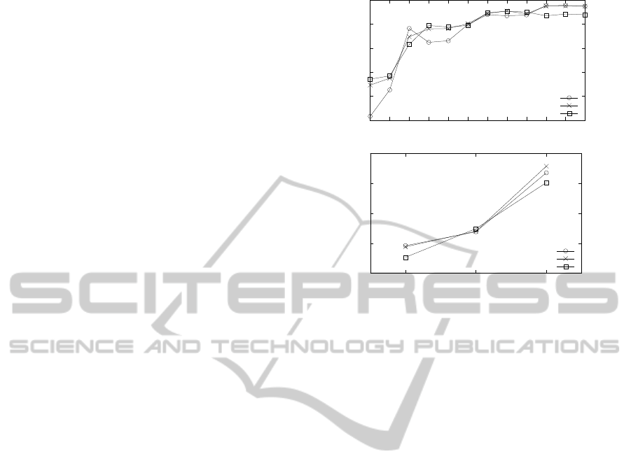
Fig. 7 shows the speedup for the Tiger and the
UAV domain with different problem sizes. Overall,
the speed up in planning optimally increases as the
sizes of the level 1 and level 0 planning problems
increase. Varying the number of candidate models
(DIDs) ascribed to the other agent did not signifi-
!"#$"%%
&'&(
&'&(
&'&(
!" #$#%
&'&($%
&'&()
&'&(%
Figure 8: The speedup for the multiagent tiger problem and
the UAV problem given different amount of level 0 models
and number of decision horizons.
cantly impact the speed ups. This is expected as
the lower-level models are solved sequentially. Par-
allelization of their solutions seems to be an obvious
avenue of future work, but is deceptively challenging.
7.2 Optimizing Thread Block Size
By parallelizing the computation on the GPU, we ob-
served around an order of magnitude speedup through
the performed experiments. As computation tasks
are organized as a set of thread blocks and exe-
cuted on SMs, the number of thread blocks deter-
mines the overall performance. Generally speaking,
more thread blocks will increase the degree of par-
allelization with higher synchronization cost. Auto-
matically calculating the optimal thread-block sizes
(Sano et al., 2014), which is domain dependent, is
beneficial but computationally expensive. The ex-
pense may be amortized over multiple runs. But, be-
cause we solve I-DIDs just once for a domain, this
expense cannot be amortized and significantly adds
to the run time. As a trade-off, we empirically search
for a block size that optimizes the solution for many
problem domains following the CUDA optimization
heuristics.
We evaluated the performance of Parallelized I-
DID Exact as the number of threads in each block
is increased from 64 to 640, on a level 1 I-DID of
horizon 3 and 10 lower-level DIDs as candidate mod-
els. The impact of different blocks sizes on run time
is shown in Fig. 9. As observed, the block size of
512 gives the best performance in terms of running
ICAART2015-InternationalConferenceonAgentsandArtificialIntelligence
192
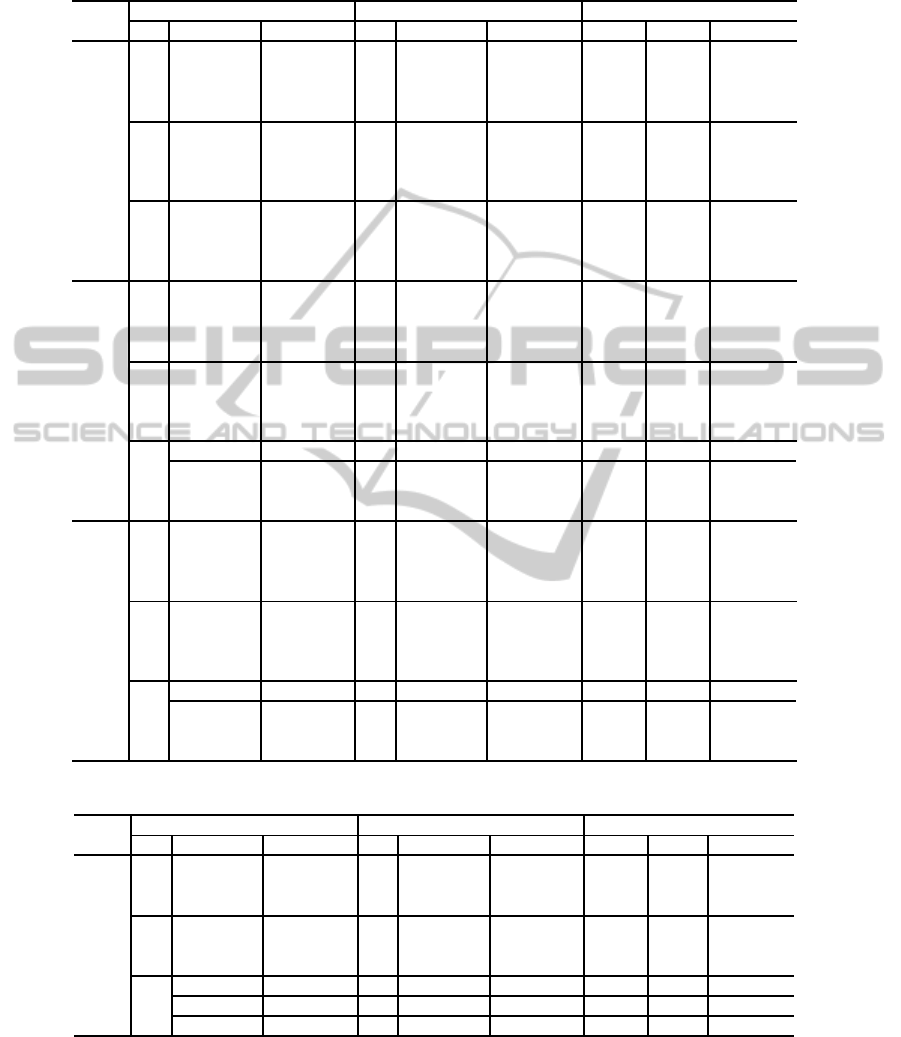
Table 1: Run times, factor sizes and speed ups for the multiagent tiger problem. |M
j
| denotes the number of level 0 models.
Mean |φ| and Mean |ψ| are the average sizes of probability and utility factors in the models, respectively. Columns titled by
CPU and GPU denote the running times for different implementations. The speedups are listed in the last column.
|M
j
|
Level 1 Level 0 Time (seconds)
T
1
Mean |φ| Mean |ψ| T
0
Mean |φ| Mean |ψ| CPU GPU Speedup
10
3 1959 2237
6 2192 1703 3.14 0.51 6.2
7 11126 8620 17.8 1.93 9.2
8 58835 45556 106 10.2 10.4
9 306284 237130 644 60.0 10.8
4 38376 44998
6 2192 1703 5.59 0.77 7.3
7 11126 8620 20.3 2.18 9.3
8 58835 45556 108 10.5 10.3
9 306284 237130 647 60.0 10.8
5 600493 655141
6 2192 1703 50.0 5.09 9.8
7 11126 8620 64.7 6.48 10.0
8 58835 45556 153 14.7 10.4
9 306284 237130 691 64.3 10.7
50
3 5449 5307
6 2192 1703 13.7 1.83 7.5
7 11126 8620 80.5 8.21 9.8
8 58835 45556 481 46.0 10.5
9 306284 237130 2930 272 10.8
4 63225 65249
6 2192 1703 16.1 2.08 7.7
7 11126 8620 83.0 8.45 9.8
8 58835 45556 484 45.9 10.5
9 306284 237130 2931 272 10.7
5
672794 683530 6 2192 1703 60.5 6.44 9.4
879830 910980
7 11126 8620 127 12.7 10.0
8 58835 45556 528 50.6 10.4
9 306284 237130 2972 277 10.7
100
3 5546 5322
6 2192 1703 27.4 3.56 7.7
7 11126 8620 162.5 16.3 9.9
8 58835 45556 971 92.8 10.4
9 306284 237130 5937 573 10.3
4 63294 65260
6 2192 1703 29.9 3.81 7.8
7 11126 8620 164.9 16.7 9.8
8 58835 45556 974 92.4 10.5
9 306284 237130 5937 569.6 10.7
5
672848 683538 6 2192 1703 74.3 8.11 9.2
879884 910989
7 11126 8620 209 21.0 9.9
8 58835 45556 1018 96.8 10.5
9 306284 237130 5975 575 10.4
Table 2: Run times, factor sizes and speed ups for the multiagent UAV problem. Columns have similar meanings.
|M
j
|
Level 1 Level 0 Time (seconds)
T
1
Mean |φ| Mean |ψ| T
0
Mean |φ| Mean |ψ| CPU GPU Speedup
10 3 104223 75120
3 1235 1029 16.56 2.22 7.5
4 20237 9467 24.38 3.17 7.7
5 392043 170405 239 27.6 8.7
25 3 106410 75270
3 1235 1029 16.9 2.27 7.4
4 20237 9467 32.6 4.23 7.7
5 392043 170405 462.4 55.6 8.8
50 3
209573 117520 3 1235 1029 17.51 2.41 7.3
212260 117695 4 20237 9467 46.61 6.02 7.7
153348 81195 5 392043 170405 845.1 99.3 8.5
time. The upside is that as more threads are involved
in the computation there are less iterations of fetching
global memory loads to shared memory. In contrast,
the degradation in performance is expected because
spawning more threads per block limits the number
of blocks that can be scheduled to run concurrently
because of limited resources, hence, the observed fall
in performance.
FastSolvingofInfluenceDiagramsforMultiagentPlanningonGPU-enabledArchitectures
193

Figure 9: The running time of the multiagent tiger problem
given different GPU’s thread block sizes.
8 CONCLUSION
We presented a method for optimal planning in multi-
agent settings under uncertainty that utilizes the paral-
lelism provided by a heterogeneous CPU-GPU com-
puting architecture. We focused on the interactive
dynamic influence diagrams, which are probabilis-
tic graphical models whose solution involves trans-
forming the I-DID into a flat DID and computing the
policy with the maximum expected utility. Opera-
tions involving probability and utility factors during
variable elimination are parallelized on GPUs. We
demonstrate speed ups close to an order of magnitude
on multiple problem domains and run times that are
less than 17 minutes for large numbers of models and
long horizons. To the best of our knowledge, these
are the fastest run times reported so far for exactly
solving I-DIDs and other related frameworks such
as I-POMDPs for multiagent planning, and represent
a significant step forward in making these complex
frameworks practical.
As aforementioned, lower level models can be
DIDs or I-DIDs with different initial beliefs. These
candidate models are differinghypotheses of the other
agent’s behavior, and therefore may be solved inde-
pendently in parallel. However, as solving I-DIDs
requires large amount of memory, we may not solve
these in parallel on a single GPU. Nevertheless, mod-
ern computing platforms may contain two or more
GPU units linked together and programmable using
CUDA.
2
Furthermore, multiple networked machines
with GPUs may be utilized using CUDA-MPI. How-
ever, as the factor operation is not computational in-
tensive, whether the saving from the parallel compu-
tation on the GPU side can compensate the cost of
transporting data between CPU and GPU is still an
2
NVIDIA promotes having multiple GPU units man-
aged by its scalable link interface.
open question. Comparisons based on different types
of GPUs will be our immediate future work as well.
ACKNOWLEDGEMENTS
This research is supported in part by an ONR Grant,
#N000141310870, and in part by an NSF CAREER
Grant, #IIS-0845036. We thank Alex Koslov for mak-
ing his implementation of a parallel Bayesian network
inference algorithm available to us for reference.
REFERENCES
Bernstein, D. S., Givan, R., Immerman, N., and Zilberstein,
S. (2002). The complexity of decentralized control of
Markov decision processes. Mathematics of Opera-
tions Research, 27(4):819–840.
Berstein, D. S., Hansen, E. A., and Zilberstein, S. (2005).
Bounded policy iteration for decentralized POMDPs.
In IJCAI, pages 1287–1292.
Chandrasekaran, M., Doshi, P., Zeng, Y., and Chen, Y.
(2014). Team behavior in interactive dynamic influ-
ence diagrams with applications to ad hoc teams. In
AAMAS, pages 1559–1560.
Chen, Y., Hong, J., Liu, W., Godo, L., Sierra, C., and
Loughlin, M. (2013). Incorporating PGMs into a BDI
architecture. In PRIMA, pages 54–69.
Doshi, P., Zeng, Y., and Chen, Q. (2009). Graphical models
for interactive POMDPs: Representations and solu-
tions. JAAMAS, 18(3):376–416.
Gal, K. and Pfeffer, A. (2008). Networks of influence di-
agrams: A formalism for representing agents’ beliefs
and decision-making processes. JAIR, 33:109–147.
Gmytrasiewicz, P. J. and Doshi, P. (2005). A framework
for sequential planning in multiagent settings. JAIR,
24:49–79.
Howard, R. A. and Matheson, J. E. (1984). Influence dia-
grams. In Howard, R. A. and Matheson, J. E., editors,
The Principles and Applications of Decision Analysis.
Strategic Decisions Group, Menlo Park, CA 94025.
Jeon, H., Xia, Y., and Prasanna, K. V. (2010). Parallel ex-
act inference on a cpu-gpgpu heterogenous system. In
ICPP, pages 61–70.
Koller, D. and Friedman, N. (2009). Probabilistic Graphi-
cal Models: Principles and Techniques. MIT Press.
Koller, D. and Milch, B. (2001). Multi-agent influence dia-
grams for representing and solving games. In IJCAI,
pages 1027–1034.
Luo, J., Yin, H., Li, B., and Wu, C. (2011). Path planning
for automated guided vehicles system via I-DIDs with
communication. In ICCA, pages 755 –759.
Pearl, J. (1998). Probabilistic Reasoning in Intelligent Sys-
tems: Networks of Plausible Inference. Morgan Kauf-
mann, Berlin, Germany.
Sano, Y., Kadono, Y., and Fukuta, N. (2014). A perfor-
mance optimization support framework for gpu-based
traffic simulations with negotiating agents. In ACAN.
ICAART2015-InternationalConferenceonAgentsandArtificialIntelligence
194

Smallwood, R. and Sondik, E. (1973). The optimal con-
trol of partially observable Markov decision processes
over a finite horizon. Operations Research, 21:1071–
1088.
Søndberg-Jeppesen, N., Jensen, F. V., and Zeng, Y. (2013).
Opponent modeling in a PGM framework. In AAMAS,
pages 1149–1150.
V. Kozlov, A. and Pal Singh, J. (1994). A parallel Lauritzen-
Spiegelhalter algorithm for probabilistic inference. In
Supercomputing, pages 320–329.
Xia, Y. and Prasanna, K. V. (2008). Parallel exact inference
on the cell broadband engine processor. In SC, pages
1–12.
Zeng, Y. and Doshi, P. (2012). Exploiting model equiva-
lences for solving interactive dynamic influence dia-
grams. JAIR, 43:211–255.
Zheng, L., Mengshoel, O. J., and Chong, J. (2011). Be-
lief propagation by message passing in junction trees:
Computing each message faster using gpu paralleliza-
tion. In UAI.
FastSolvingofInfluenceDiagramsforMultiagentPlanningonGPU-enabledArchitectures
195
