Multi-start Iterated Local Search for Two-echelon Distribution Network

for Perishable Products

S. Kande

1,2

, C. Prins

, L. Belgacem

and B. Redon

ICD-LOSI, University of Technology of Troyes, 12 rue Marie Curie, CS 42060, 10004 Troyes Cedex, France

FuturMaster, 1 cours de l’ile seguin, 92100 Boulogne-Billancourt, France

Keywords:

Distribution network, Multi-Start Iterated Local Search, Local Search, Lot-sizing, Metaheuristic, Multi-

echelon inventory, Multi-sourcing, Perishable product, Supply planning, Transport capacity, Variable

neighborhood descent.

Abstract:

This article presents a planning problem in a distribution network incorporating two levels inventory man-

agement of perishable products, lot-sizing, multi-sourcing and transport capacity with a homogeneous ﬂeet of

vehicles. A mixed integer linear programming (MILP) and a greedy heuristic were developed to solve this real

planning problem. There are some instances for which the solver cannot give a good lower bound within the

limited time and for other instances it takes a lot of time to solve MILP. The greedy heuristic is an alternative

to the mixed integer linear program to quickly solve some large instances taking into account original and

difﬁcult constraints. For some instances the gap between the solutions of the solver (MILP) and the heuris-

tic becomes quite signiﬁcant. A multi-start iterated local search (MS-ILS), using the variable neighborhood

descent (VND) and a greedy randomized heuristic, has been implemented. It has been included in an APS

(Advanced Planning System) and compared with an exact resolution of the MILP. The instances are derived

from actual data or built using a random generator of instances to have wider diversity for computational

evaluation. The MS-ILS signiﬁcantly improves the quality of solutions.

1 INTRODUCTION

In the problem under study, warehouses provide ﬁn-

ished perishable products to various distribution cen-

ters with a homogeneous ﬂeet of vehicles. A distri-

bution center may be supplied by several warehouses.

The choice of sourcing (warehouse) is determined by

the availability of products in warehouses inventory,

ﬂeet of vehicles, and transport costs on roads. The

goal is to come up with a compromise between the

transportation costs, the warehouses and distribution

centers inventory costs, the loss due to products that

are outdated. Furthermore, we comply with: ﬂow

conservation, inventory conservation at warehouses

and distribution centers, capacity constraints (limited

ﬂeet of vehicles on each road) and supply constraints

(lot-sizing, minimum order quantities and dates).

The remainder of this article is structured as fol-

lows. In Section 2, we present a literature review. The

problem addressed in the paper is described in Section

3. We explain how the multi-start iterated local search

has been implemented in Section 5. Section 6 is ded-

icated to computational experiments and comparison

with solver solution (MILP) and greedy heuristic. The

last section (7) gives the next steps of the work.

2 LITERATURE REVIEW

Iterated local search (ILS) method is a popular heuris-

tic in the literature. (Lourenc¸o et al., 2003) present a

tutorial about the ILS method and its application to

some problems such as the travelling salesman prob-

lem and the scheduling, and compare the ILS with

other metaheuristics; also with another recent paper

(Lourenc¸o et al., 2010).

(Cuervo et al., 2014) recently propose an ILS for the

vehicle routing problem with backhauls (VRPB). It

is an extension of the VRP that deals with two types

of customers: the consumers (linehaul) that request

goods from the depot and the suppliers (backhaul)

that send goods to the depot. New best solutions have

been found by the authors for two instances in one of

the benchmark sets. A multi-start iterated local search

(MS-ILS) is developed by (Nguyen et al., 2012) for

294

Kande S., Prins C., Belgacem L. and Redon B..

Multi-start Iterated Local Search for Two-echelon Distribution Network for Perishable Products.

DOI: 10.5220/0005224902940303

In Proceedings of the International Conference on Operations Research and Enterprise Systems (ICORES-2015), pages 294-303

ISBN: 978-989-758-075-8

 2015 SCITEPRESS (Science and Technology Publications, Lda.)

the two-echelon location-routing problem (LRP-2E).

They use three greedy randomized heuristics (cycli-

cally to get initial solutions), the variable neighbor-

hood descent and a tabu list. MS-ILS is also used by

(Michallet et al., 2014) for the periodic vehicle rout-

ing problems with time spread constraints on services.

Their paper addresses a real-world problem. The time

windows must be absolutely respected and the hours

of any two visits to the same customer must differ by

a given time constant. They make evaluations on in-

stances derived from classical benchmarks for the ve-

hicle routing problem with time windows, and on two

practical instances. For a particular case with a sin-

gle period (the vehicle routing problem with soft time

windows), MS-ILS competes with two published al-

gorithms and improves six best known solutions.

The greedy randomized adaptive search procedure

(GRASP) (Feo and Bard, 1989) (Feo and Resende,

1995) is a memory-less multi-start method in which

local search is applied to different initial solutions

constructed with a greedy randomized heuristic. (Vil-

legas et al., 2010) propose two metaheuristics based

on greedy randomized adaptive search procedures

(GRASP), variable neighborhood descent (VND) and

evolutionary local search (ELS). The problem under

study is the single truck and trailer routing problem

with satellite depots (STTRPSD): a vehicle composed

of a truck with a detachable trailer serves the demand

of a set of customers reachable only by the truck with-

out the trailer. The accessibility constraint implies the

selection of locations to park the trailer before per-

forming the trips to the customers. The computational

experiment shows that a multi-start evolutionary local

search (GRASP-ELS) outperforms a GRASP/VND.

Moreover, it obtains competitive results when ap-

plied to the multi-depot vehicle routing problem, that

can be seen as a special case of the STTRPSD. The

GRASP-ELS is also used by (Duhamel et al., 2011)

for an extension of the capacitated vehicle routing

problem where customer demand is composed of two-

dimensional weighted items (2L-CVRP). The results

show that their method is highly efﬁcient and out-

performs the best previous published methods on the

topic.

We have not found any paper that proposes multi-

start iterated local search method for the problem un-

der study.

3 PROBLEM DESCRIPTION

The distribution network considered includes two lev-

els: warehouses that provide perishable products to

several distribution centers (see Figure 1). A distri-

Figure 1: Two echelon distribution network with multi-

sourcing.

bution center may be supplied by several warehouses.

The choice of the sourcing (warehouse) is determined

by the products availability in warehouses inventory,

transport capacity and transport costs on the roads.

The out of stock is permitted at the distribution cen-

ters; unmet demand may be postponed but is penal-

ized by a cost. Stock levels are taken into account in

the end of period. Every product shipped in a road has

an associated cost of transport which determines the

priority level of the warehouse. For each product-site

(product-warehouse and product-distribution center)

a stock policy is deﬁned by three elements:

• a variable target stock in time: ideally reach tar-

get;

• a variable maximum stock in time: limit beyond

which there is an overstock and product poses a

risk of obsolescence;

• a variable minimum stock in time: reserve to cope

with ﬂuctuations in demand.

Products are made in batches to the warehouse.

To differentiate with the concept of design in batches,

“ batch ” stands for the set of product characterized

by an amount of one type of product, the input date

into the stock and expiry date. For each warehouse

the batches of products are ordered in ascending or-

der of their expiry dates and consumption occurs in

this order. In addition, a freshness contract of prod-

uct is made between the distribution center and their

customers. It is a remaining life at least at the delivery

time to the customer (at the period of distribution cen-

ter requirement). A distribution center requirement

can be satisﬁed by several batches of the same prod-

uct. When a batch is not consumed before its expiry

date then there is a loss of the remaining amount. It is

penalized by a cost called waste cost.

Constraints of lot size and a minimum supply

quantity must be respected. The minimum quantity

expresses an economic quantity necessary for prof-

itable order launch and reception operations. The lot

size constraint corresponds sending by pallets for the

transport. The combination of these two constraints

(lot size and minimum quantity) makes this much

Multi-startIteratedLocalSearchforTwo-echelonDistributionNetworkforPerishableProducts

295

more complex than classical multi-echelon inventory

management problems. A shipping calendar (opening

or closing depending on the period) is also deﬁned on

each transport road.

The supply planning shall establish the quantities

for each product and period to deliver to warehouses

and distribution centers to satisfy at best the require-

ments (distribution centers) and reach the target stock

(warehouses and distribution centers). The objective

is to minimize the costs of transport, warehouses stor-

age and distribution centers storage, the loss due to

product obsolescence, out of stock penalties and tar-

diness penalties. We must respect the ﬂow’s coher-

ence, the capacity constraints, the supply constraints

(lot size, minimum quantity and dates) and seek to

optimize the balancing of multi-echelon stock.

For reasons of ﬂexibility, the user has the possi-

bility of imposing quantity to supply inventory ware-

houses, distribution centers, also for transport. It is

used to circumvent the various constraints in a crit-

ical situation. However, it can lead to inconsisten-

cies in the calculation. During the execution of these

heuristics, the inconsistencies are detected and re-

ported without interrupting the supply planning calcu-

lation; which cannot be mixed with the MILP solver.

4 MATHEMATICAL MODEL

The problem can be formulated as a mixed integer lin-

ear programming. There are K warehouses (indexed

by k), L distribution centers (indexed by l), P prod-

ucts (indexed by p), T number of periods of hori-

zon of calculation (indexed by t), U number of pe-

riods of horizon of expiry dates (indexed by u) as

u ∈ 1, ..., T + max(DLU

). All indexes start at 1 ex-

cept the stock levels sd

l pt

, sw

kpt

for which the index

starts at 0 for the initial stock. Constraints use a large

positive constant M.

4.1 Notations

The names of the data is in upper-case and those vari-

ables in lower-case.

l pt

∈ IR

, l ∈ L, p ∈ P, t ∈ T : customer requirement of

the product p at the distribution center l at the period

t ;

Data for the Supply and the Shipment:

min

ipt

∈ IN, i ∈ K ∪ L, p ∈ P, t ∈ T : minimum quantity

of the product p to supply at the warehouse/distribution

center i at the period t;

kpt

∈ {0, 1}, k ∈ K, p ∈ P, t ∈ T : shipment calendar; if

kpt

= 1 the product p can be shipped from the ware-

house k at the period t;

l pt

∈ {0, 1}, l ∈ L, p ∈ P, t ∈ T : reception calendar; if

l pt

= 1 the product p can be receipt at the distribu-

tion center l at the period t;

DLU

∈ IN : number of periods the quantity of the prod-

uct p, supplied at the warehouse k, can be used : after

this lead time the product is expired ;

MCL

l pt

∈ IN : minimum customer life is a remaining life-

time, at least, when the product p is delivered to the

customer from the distribution center l at the period t);

FPO

ipt

∈ IR

: ﬁrm planned order is a quantity of

the product p imposed by the user at the ware-

house/distribution center i at the period t;

IsFPO

ipt

∈ {0, 1} : IsFPO

ipt

= 1 if there is a quantity

of the product p imposed by the user at the ware-

house/distribution center i at the period t, so we can not

supply a different quantity for the same product at this

time (the value zero is considered);

QEID

l pt

∈ IR

: quantity of the product p receipt at the

distribution center l at the period t from a external

sourcing.

Data for the Inventory:

init

∈ IR

, i ∈ K ∪ L, p ∈ P : initial stock level of the

product p at the warehouse/distribution center i ;

ob j

ipt

∈ IR

, i ∈ K ∪ L, p ∈ P, t ∈ T : target stock level of

the product p at the warehouse/distribution center i at

the period t;

max

ipt

∈ IR

, i ∈ K ∪ L, p ∈ P, t ∈ T : maximum stock level

of the product p at the warehouse/distribution center i

at the period t ;

min

ipt

∈ IR

, i ∈ K ∪ L, p ∈ P, t ∈ T : minimum stock level

of the product p at the warehouse/distribution center i

at the period t ;

>max

ipt

∈ IR

, i ∈ K ∪ L, p ∈ P, t ∈ T : unit penalty of

overstock if we exceed the maximum stock level of the

product p at the warehouse/distribution center i at the

period t (per unit of surplus stock);

>ob j

ipt

∈ IR

, i ∈ K ∪ L, p ∈ P, t ∈ T : unit earliness

penalty when the stock level, of the product p at

the warehouse/distribution center i at the period t, is

between the target stock and the maximum stock;

<ob j

ipt

∈ IR

, i ∈ K ∪ L, p ∈ P, t ∈ T : unit tardiness

penalty when the stock level, of the product p at

the warehouse/distribution center i at the period t, is

between the minimum stock and the target stock (by

missing unit to reach the target stock);

<min

ipt

∈ IR

, i ∈ K ∪ L, p ∈ P, t ∈ T : unit penalty applied

when the stock level, of the product p at the ware-

house/distribution center i at the period t, is between

0 and the minimum stock (by missing unit to reach the

minimum stock);

rupt

l pt

∈ IR

, l ∈ L, p ∈ P, t ∈ T : unit penalty of out of

stock applied when the stock level, of the product p at

the distribution center l at the period t, is under 0 (the

out of stock is only permitted at the distribution cen-

ters);

ICORES2015-InternationalConferenceonOperationsResearchandEnterpriseSystems

296

obs

kpt

∈ IR

, k ∈ K, p ∈ P, t ∈ T : unit penalty of obsoles-

cence of the product p at the warehouse k at the period

t (the lifetime is is exceeded).

Data for the Transport:

QTA

min

kl pt

∈ IN : minimum quantity of the product p shipped

on edge (k, l) at the period t;

T L

kl p

∈ IN : lot size for the shipment of the product p on

the edge (k, l) in units of product;

kl pt

∈ {0, 1} : CT

kl pt

= 1 if the transport of the product

p is permitted on the edge (k, l) at the period t;

klt

∈ IN, k ∈ K, l ∈ L, t ∈ T : available capacity on the

edge (k, l) at the period t, expressed as the number of

pallets;

CoPa

∈ IR

, p ∈ P : conversion factor quantity → pallets

of the product p;

∈ IR

, k ∈ K, l ∈ L : cost of operating a vehicle on

the edge (k, l) (counted only once even if the vehicle

travelled several days);

kl pt

∈ IR

, k ∈ K, l ∈ L, p ∈ P, t ∈ T : unit cost of the

shipment of the product p on the edge (k, l) at the pe-

riod t;

klt

∈ IN, k ∈ K, l ∈ L, t ∈ T : lead time of transport on

the edge (k, l) at the period t;

max

∈ IN : maximum number of pallets a vehicle can be

loaded (same for all vehicles);

max

∈ IR

: maximum loading weight of a vehicle

(same for all vehicles);

∈ IR

, p ∈ P : unit weight of the product p;

FPOA

kl pt

∈ IR

: quantity imposed to ship the product p

on the edge (k, l) at the period t (useful for imposing an

origin and a destination);

IsFPOA

kl pt

∈ {0, 1} : IsFPOA

kl pt

= 1 if there is a quantity

imposed to ship the product p on the edge (k, l) at the

period t ([FPOA

kl pt

;

max

klt

, k ∈ K, l ∈ L, t ∈ T : number of vehicles used on the

edge (k, l) at the period t.

Variables for the Supply and the Shipment:

ipt

, i ∈ K ∪ L, p ∈ P, t ∈ T : quantity of the product p

supplied at warehouse/distribution center i at the period

isqi

ipt

∈ {0, 1}, i ∈ K ∪ L, p ∈ P, t ∈ T : isqiw

ipt

= 1 if a

non-zero quantity of the product p is supplied at ware-

house/distribution center i at the period t;

kpt

, k ∈ K, p ∈ P, t ∈ T : quantity of the product p

shipped by warehouse k at the period t (output quan-

tity);

kpt

, k ∈ K, p ∈ P, t ∈ T : quantity of the product p lost

due to obsolescence at the warehouse k at the period t;

kl pt

∈ IN, k ∈ K, l ∈ L, p ∈ P, t ∈ T : number of lots that

form the quantity shipped on the edge (k, l) at the period

kl pt

, k ∈ K, l ∈ L, p ∈ P, t ∈ T : quantity of the product

p shipped on the edge (k, l) at the period t;

isqe

kl pt

∈ {0, 1}, k ∈ K, l ∈ L, p ∈ P, t ∈ T : isqe

kl pt

= 1 if

a non-zero quantity of the product p is shipped on the

edge (k, l) at the period t;

qed

kl pu

, k ∈ K, l ∈ L, p ∈ P, u ∈ U : total quantity of the

product p shipped on the edge (k, l) and whose expi-

ration date is u;

qed p

kl ptu

, k ∈ K, l ∈ L, p ∈ P, t ∈ T , u ∈ U : quantity of

the product p shipped on the edge (k, l) at the period t

and whose expiration date is u;

qoi

kl pt

, k ∈ K, l ∈ L, p ∈ P, t ∈ T : quantity of the product

p shipped by the warehouse k and receipt at the distri-

bution center l at the period t .

Variables for the Inventory:

sdlu

kpu

: quantity of the product p and whose expiration

date is u at the warehouse k;

ipt

, i ∈ K ∪ L, p ∈ P, t ∈ T : stock level of the product p at

the warehouse k at the period t;

rupt

l pt

, l ∈ L, p ∈ P, t ∈ T : missing quantity to avoid the out

of stock when the stock level is negative;

<min

ipt

, i ∈ K ∪ L, p ∈ P, t ∈ T : missing quantity to reach

the minimum stock, from 0 until the minimum stock;

<ob j

ipt

, i ∈ K ∪ L, p ∈ P, t ∈ T : missing quantity to reach

the target stock, from the minimum stock until the tar-

get stock;

>ob j

ipt

, i ∈ K ∪ L, p ∈ P, t ∈ T : quantity between the stock

level and the target stock, from the target stock until the

maximum stock;

>max

ipt

, i ∈ K ∪ L, p ∈ P, t ∈ T : quantity between the stock

level and the maximum stock, when the stock level is

over the maximum stock.

4.2 Stock Cost Formulation

Two cost functions, whose shape is shown in the ﬁg-

ure 2, are deﬁned to evaluate the inventory of the

warehouses and the distribution centers. The func-

tion f (s

ipt

) means the stock cost of the product p in

the warehouse/distribution center i at time t. This

is a piecewise linear convex function. It has a zero

value when the stock level is equal to the target stock.

This corresponds to a cost of storage and optionally

of overstock (stock level greater than the maximum

stock) when the stock level is above the target stock.

When the stock level is lower than the target stock, it

is the cost of delay and possible risk of out of stock

(stock level below the minimum stock). For the dis-

tribution centers, a penalty for negative stock (cost of

out of stock) is added.

Illustrated in the ﬁgure 3, the variables of gap are

deﬁned to linearise the piecewise linear functions.

These are the quantities of gap for each piece.

Cost functions of stock at the warehouses and the

Multi-startIteratedLocalSearchforTwo-echelonDistributionNetworkforPerishableProducts

297

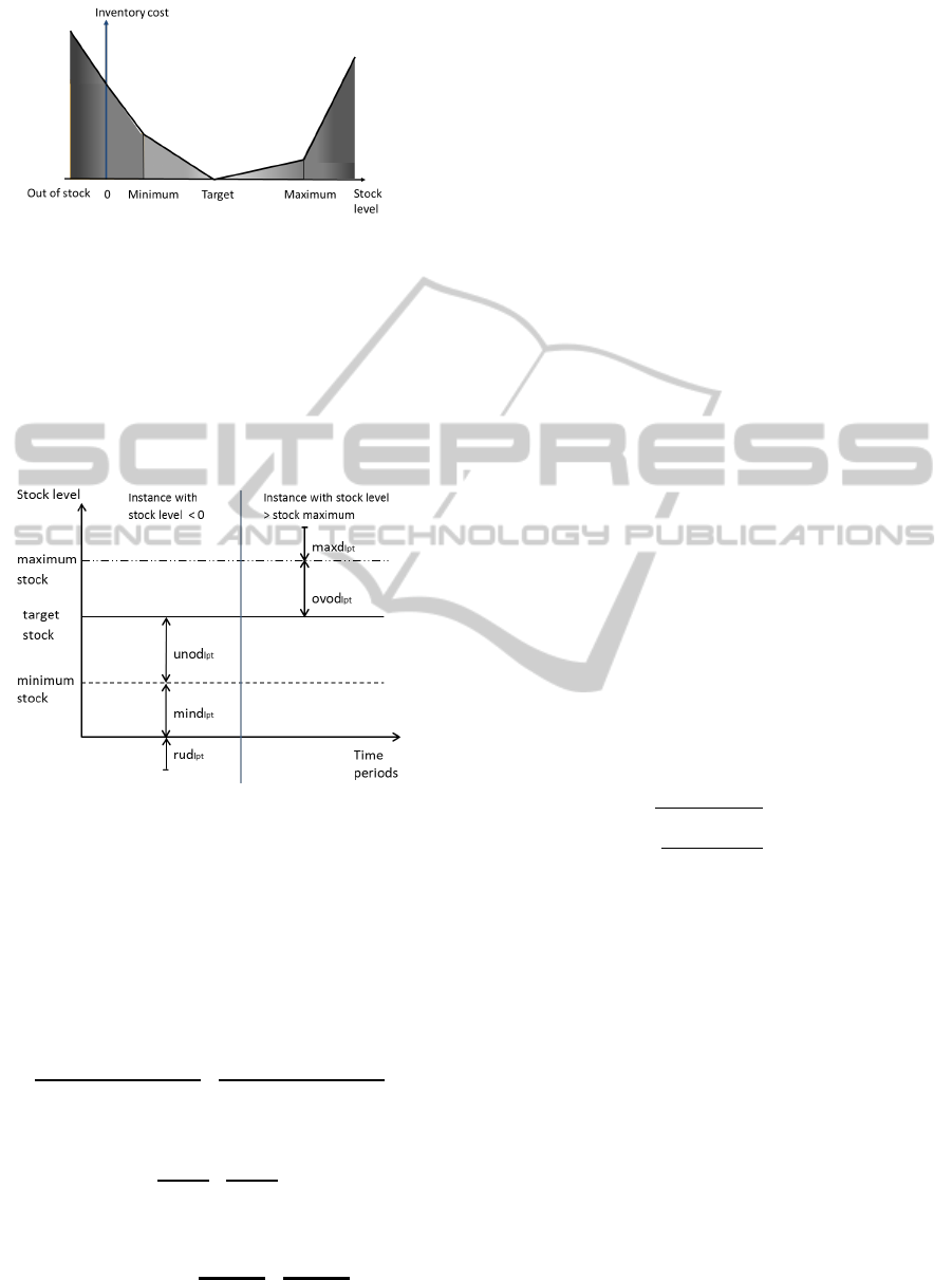
Figure 2: Stock policy and the penalties.

distribution centers may be formulated as follows:

f (s

ipt

) =

(

rupt

l pt

· s

rupt

l pt

+ P

<min

ipt

· s

min

ipt

+ P

<ob j

ipt

· s

<ob j

ipt

>ob j

ipt

· s

>ob j

ipt

+ P

>max

ipt

· s

>max

ipt

Figure 3: Variables for linearisation of the piecewise linear

functions.

4.3 MILP Formulation

Objective function:

Min Z = (1)

∑

k=1

∑

l=1

∑

t=1

(HV

· v

max

klt

) +

∑

p=1

(qe

kl pt

· HT

kl pt

)

| {z }

transport cost

K∪L

∑

i=1

∑

p=1

∑

t=1

f (s

ipt

)

| {z }

warehouses and distribution centers stock cost

∑

k=1

∑

p=1

∑

t=1

obs

kpt

· qp

kpt

{z }

cost of loss due to obsolescence

subject to:

kl pt

= F POA

kl pt

if IsFPOA

kl pt

= 1 ∀k ∀l ∀p ∀t (2)

kl pt

= n

kl pt

· T L

kl p

if IsFPOA

kl pt

= 0, T L

kl p

6= 0 ∀k ∀l ∀p ∀t (3)

kl pt

≥ isqe

kl pt

· (1 − IsFPOA

kl pt

) · QTA

min

kl pt

∀k ∀l ∀p ∀t (4)

kl pt

≤ isqe

kl pt

· M ∀k ∀l ∀p ∀t (5)

kl pt

= qe

kl pt

·CT

kl pt

if IsFPOA

kl pt

= 0 ∀k ∀l ∀p ∀t (6)

qoi

kl p,t+LT

klt

= qe

kl pt

∀k ∀l ∀p ∀t (7)

ipt

= F PO

ipt

if IsFPO

ipt

= 1 ∀i ∀p ∀t (8)

ipt

≥ isqi

ipt

· (1 − IsFPO

ipt

) · QT

min

ipt

∀i ∀p ∀t (9)

ipt

≤ isqi

ipt

· M ∀i ∀p ∀t (10)

l pt

= CRD

l pt

∑

k=1

qoi

kl pt

if IsFPO

ipt

= 0 ∀l ∀p ∀t > LT

klt

(11)

kpt

= CE

kpt

∑

l=1

kl pt

∀k ∀p ∀t (12)

ip0

= S

init

∀i ∀p (13)

kpt

= sw

kpt−1

+ qi

kpt

− qo

kpt

∀k ∀p ∀t > 0 (14)

l pt

= sd

l pt−1

+ qi

l pt

+ QEID

l pt

− D

l pt

∀l ∀p ∀t > 0 (15)

swdlu

kpu

= 0 ∀k ∀p ∀u < DLU

(16)

swdlu

kpu

= S

init

∀k ∀p u = DLU

(17)

swdlu

kpu

= qi

kpt

∀k ∀p ∀t

u = t + DLU

(18)

kl pt

∑

u=1

qed p

kl ptu

∀k ∀l ∀p

∀t >= u − DLU

(19)

qed

kl pu

∑

t=1

qed p

kl ptu

∀k ∀l ∀p ∀u (20)

∑

l=1

qed

kl pu

≤ swdlu

kpu

∀k ∀p ∀u (21)

∑

u=1

qed

kl pu

≤

∑

t=1

l pt

∀k ∀l ∀p ∀u ≤ T

∀t ≤ u − MCL

l pt

(22)

kpt

= swdlu

kpu

−

∑

l=1

qed

kl pu

∀k ∀p ∀t = u (23)

klt

≥ v

max

klt

· NPmax ∀k ∀l ∀t (24)

max

klt

≥

∑

p=1

kl pt

·COPA

NPmax

∀k ∀l ∀t (25)

max

klt

≥

∑

p=1

(qe

kl pt

· PU

)

PV max

∀k ∀l ∀t (26)

rupt

l pt

≥ 0 − s

l pt

∀l ∀p ∀t (27)

<min

ipt

rupt

l pt

≥ S

min

ipt

− s

ipt

∀i ∀p ∀t (28)

<ob j

ipt

+ s

<min

ipt

rupt

l pt

≥ S

ob j

ipt

− s

ipt

∀i ∀p ∀t (29)

>ob j

ipt

+ s

>max

ipt

≥ s

ipt

− S

ob j

ipt

∀i ∀p ∀t (30)

>max

ipt

≥ s

ipt

− S

max

ipt

∀i ∀p ∀t (31)

kpt

, swdlu

kpu

≥ 0 ∀k ∀p ∀t ∀u (32)

l pt

∈ IR ∀l ∀p ∀t (33)

kl pt

∈ IN ∀k ∀l ∀p ∀t (34)

kpt

, qp

kpt

, qi

ipt

, qe

kl pt

, qoi

kl pt

, qed

kl pu

qed p

kl ptu

≥ 0 ∀i ∀k ∀l ∀p ∀t ∀u(35)

max

klt

∈ IN ∀k ∀l ∀t (36)

isqe

kl pt

, isqi

ipt

∈ {0, 1} ∀k ∀l ∀p ∀t (37)

rupt

l pt

≥ 0 ∀l ∀p ∀t (38)

<min

ipt

, s

<ob j

ipt

, s

>ob j

ipt

, s

>max

ipt

≥ 0 ∀i ∀p ∀t (39)

The objective function (1) includes the transport

costs, the costs of stock for the warehouses and dis-

tribution centers, the cost of loss due to obsolescence.

The constraints (2) and (8) ensure that the imposed

ICORES2015-InternationalConferenceonOperationsResearchandEnterpriseSystems

298

quantities are respected. The lot size of the shipped

quantities is respected via the constraint (3). Con-

straints (4), (5), (9) and (10) concern the minimum

quantities for the receipt quantities at the distribution

centers and the warehouses, and the shipped quanti-

ties on the routes. If there is not a imposed quantity,

we can ship if the shipping calendar is open (6). The

shipping quantity arrives at the distribution center af-

ter the lead time on the route (7). The receipt quantity

at the distribution center corresponds to the sum of

all the shipped quantities and the reception calendar

must be opened (11). The output quantity at the ware-

house is equal to the sum of all the shipped quantities

and the shipping calendar must be opened (12). Flow

conservation and the levels of inventory are expressed

via constraints (13)-(15). The inventory stock by date

of expiry is expressed via constraints (16)-(18). Con-

straints (19)-(21) concern the use of batches of quanti-

ties taking into account their expiry date. Constraints

(22) guarantee that the freshness contract (minimum

customer life) is respected. The lost quantities in the

warehouse (the batches that are not consumed before

expiry date) are calculated using constraint (23). Con-

straints (24)-(26) check that the transport capacity is

not exceeded by the number of pallets and the total

weight of shipped products. The linearisation of the

variables of gap are made with constraints (27)-(31)

for the stock at the distribution centers and the stock

at the warehouses. The variables are deﬁned in the

lines (32)-(39).

There are some instances for which the solver can-

not give a good lower bound within the limited time

and for other instances it takes a lot of time to solve

MILP. A greedy heuristic has been implemented as

an alternative to the mixed integer linear program to

quickly solve some large instances. For some in-

stances the gap between the solution provided by the

solver (MILP) and the heuristic becomes quite sig-

niﬁcant. An multi-start iterated local search (MS-

ILS) has been implemented to improve the quality of

heuristic solutions.

5 MULTI-START ITERATED

LOCAL SEARCH

The MS-ILS method uses several runs of ILS method,

which is developed with a reactive randomized

heuristic (RRH) and the variable neighborhood de-

scent (VND) method.

MS-ILS algorithm

execute 100 times the reactive randomized

heuristic to get statistics and identify

the best settings

j:= 1

Repeat

execute the ILS method

Until {j > Number_{run} or Time limit reached}.

5.1 RRH-VND

We were inspired by the papers of (Prais and Ribeiro,

2000) and, (Prins and Calvo, 2005) for the GRASP.

Prais and Ribeiro proposed reactive method GRASP

for a problem in telecommunication. Prins and

Wolﬂer Calvo also proposed a GRASP which is re-

peatedly running a greedy randomized heuristic that

improves with a local search. In our method, a greedy

heuristic is used to get initial solution and VND pro-

cedure is used to improve this solution. A greedy

heuristic has been implemented as an alternative to

the mixed integer linear program to quickly solve

some large instances. It is divided into three main

procedures to better balance stock levels. The re-

quirement of the distribution centers is ﬁrst processed

regardless of target stock: this is to determine the

amount necessary to avoid out of stock (minimum

supply process). Then, we seek to achieve the tar-

get stock. Finally, the surplus in the warehouses is

deployed to the distribution centers. This division

into three phases allows better management of cases

of shortage or very limited capacity, since it seeks to

ensure that all the distribution centers are supplied to

meet requirement, before trying to establish the target

stock.

Two types of randomization have been incorpo-

rated in the heuristic. This is the sort of list of couples

product-warehouse and the product-distribution cen-

ter.

5.1.1 Randomization of The List of Couples

Product-Warehouse

In the process of minimum supply list couples prod-

uct warehouse is sorted then traveled in order “ natu-

ral ” (each product-warehouse is indexed by its mem-

ory address). For each product-warehouse, the list of

couples supplied product-distribution center is gener-

ated. The available quantity is shared in order to avoid

out of stock (at couples product-distribution center).

The purpose of this randomization is to test different

courses from the list of couples product-warehouse.

A parameter k is deﬁned, it represents the number

of elements of the set. A couple is randomly chosen

among the k ﬁrst items on the list of couples product-

warehouse. The method is as follows:

• create a set with the ﬁrst k elements;

• randomly select an item in the set;

Multi-startIteratedLocalSearchforTwo-echelonDistributionNetworkforPerishableProducts

299

• allocate quantities to avoid breakage distribution

center product couples who purchase mainly from

the product warehouse selected;

• integrate the next element located at position k+1

in the list as a whole.

5.1.2 Randomization of The List of Couples

Product-Distribution Center

In the procurement process to achieve the target stock

of couples product-distribution center, the list of cou-

ples is sorted in order of the memory address. For

each product-distribution center, just in time supply

is made from the main sourcing (warehouse): the

unit cost of transportation and prioritizes the lowest

cost associated with the arc carrying the main ware-

house. If this treatment does not achieve the target

stock torque then distribution center product supply

options early, late and from other warehouses (sec-

ondary, tertiary, etc ...) are evaluated and applied. We

seek to disrupt the criticality associated with couples

distribution center product; which changes the sort or-

der of the list of golf couples distribution center prod-

uct. This randomization is performed as follows:

• calculate the criticality of each product-

distribution center: in the case of sorting

criteria default value of 1 is assigned to each

couple;

• randomly increase the value for each criticality of

0 to k %;

• sort the list of couples distribution center product

in descending order of criticality values obtained.

5.1.3 Variable Neighborhood Descent

(Hansen and Mladenovi

c, 2001) proposed the vari-

able neighborhood search (VNS) in which several

neighborhoods are successively used. VNS does not

follow a single trajectory but explores increasingly

distant neighbors of the incumbent and jumps from

this solution to a new one in case of improvement. Lo-

cal search is used to get from these neighbors to local

optima. VNS is based on the principle of systemati-

cally exploring several different neighborhoods, com-

bined with a perturbation move (called shaking in the

VNS literature) to escape from local optima. Variable

neighborhood descent (VND) is essentially a simple

variant of VNS, in which the shaking phase is omit-

ted. Therefore, contrary to VNS, VND is usually

completely deterministic.

The different movements used in our VND proce-

dure are more or less complex. Simple movements are

to increase or reduce the supplied amounts to the dis-

tribution centers and the warehouses. Complex move-

ments can transfer amounts from a time period to an-

other, from a distribution center to another and from

a warehouse to another. The decrease of the sup-

plied quantities (movements 1 and 6) is designed to

avoid overstock: when the stock level is above the tar-

get stock at product-site couples (product-warehouse

and product-distribution center). When applied on

a product-distribution center the quantity is spread

across the ﬂow; on the road and the sourcing (product-

warehouse). The increase of supplied quantity (move-

ments 3 and 7) can compensate for the gap when the

stock level is below the target stock level at couples

product-site. Amounts may be transferred between

different periods of the horizon for all product-site

couples (movements 2 and 9). The amount removed

from the starting period is not necessarily equal to

that added at the arrival time. An exchange can oc-

cur between two product-distribution center couples

sharing the same transport road (movement 4). The

interest of this movement is to ﬁnd a balance between

the stock levels of the different products in a distribu-

tion center using the same warehouse provider. Con-

sumption of transport capacity is not optimized by the

greedy heuristic. The quantity removed from the orig-

inal product-distribution center may be different from

the added amount. Different distribution centers sup-

plying the same product from the same warehouse are

also the subject of an exchange (movement 8). A par-

ticular movement (movement 5) is integrated to re-

duce the cost of loss due to product obsolescence in

warehouses. When the removal is possible, the lot in

question is exchanged with some or several consign-

ments to meet the needs of product-distribution cen-

ter couples. Constraints dates such as expiry date and

contract freshness are always respected.

The VND stops if no movement improves solu-

tion cost or the improvement percentage (IP) of so-

lution cost between two successive iterations is less

than 0.01%. This gap is also a stop criterion for solver

MILP resolution. The second criterion can reduce

computational time without degrading solution qual-

ity. The formula of this gap is as follows:

IP =

last solution cost - solution cost

solution cost

× 100 (40)

VND algorithm

Cost(Sol):=reactive randomized heuristic solution cost

initialise Number_{Move}

Repeat

Cost(LastSol):= Cost(Sol)

i:= 1

While {i <= Number_{Move}}

For {$N(Sol,i)$}

Sol’:= LocalSearch N(Sol,i)

If {Cost(Sol’) < Cost(Sol)}

Sol:= Sol’

EndIf

EndFor

ICORES2015-InternationalConferenceonOperationsResearchandEnterpriseSystems

300

EndWhile

Until {Cost(Sol) >= Cost(LastSol) or IP <= 0.01

or Time limit reached}.

5.2 Iterated Local Search

For (Lourenc¸o et al., 2003), ILS has many of the de-

sirable features of a metaheuristic: it is simple, easy

to implement, robust, and highly effective. The es-

sential idea of ILS lies in focusing the search not on

the full space of solutions but on a smaller subspace

deﬁned by the solutions that are locally optimal for

a given optimization engine. Each iteration, a copy

of the best known solution is disturbed and the local

search is generally used to improve it. The strength of

the method is that the solutions generated are depen-

dent and trace a path of local optima near each other

in the space of solutions. ILS is also very fast: if the

disturbance is slight enough, the new solution looks

to the parent solution and the local search needs only

few movements to re-optimize it.

In our method, a reactive randomized heuristic is

used as initial solution and variable neighborhood de-

scent (VND) is used to improve this solution. We get

a local optimum at the end of VND. At each iteration,

movements (perturbation) are executed to get a new

solution from which VND is applied. After the per-

turbation the new solution is different and less good

than the local optimum but VND can improve it and

give a better solution. ILS stops if a ﬁxed number of

iterations is reached. The higher the number of itera-

tions, the greater the computational time is.

ILS algorithm

execute VND (BestSol)

initialise shaking parameters k_{min}, k_{max}

initialise iterations number max_{iterator}

k:= k_{min}

i:= 1

Repeat

Sol:= BestSol

Shaking move (Sol)

execute VND (Sol)

If {Cost(Sol) < Cost(BestSol)}

BestSol:= Sol

k := k_{min}

Else

Sol:= BestSol

k := k + 1

If {k > k_{max}}

k := k_{min}

EndIf

Until {i > max_{iterator} or Time limit reached}.

5.2.1 Perturbation

Perturbation is a mechanism to escape from local op-

tima. Our perturbation is powered by four move-

ments. The ﬁrst is the movement of removing ob-

solete batch for product-warehouse couples. Delet-

ing obsolete batches can degrade the stock of the

warehouse over several periods; which cause an in-

crease in the stock cost and cancel the decrease in the

waste cost. When this perturbation movement is ap-

plied the change is accepted even if the cost of the

solution increases. The movement of adding quan-

tity for product-warehouse couples can correct this

effect in the next VND application. The second and

third movements are movements of decreasing quan-

tity, respectively for the product-distribution center

couples and the product-warehouse couples. These

movements are applied in VND and may cause dete-

rioration of the stock over future periods. The fourth

movement is used to exchange amounts between the

product-distribution center couples sharing the same

source. In some cases the available warehouse re-

sources is restricted to satisfy all requirements of dis-

tribution centers. Some exchanges of amounts are

made to modify the distribution made by the greedy

heuristic and let VND improve the solution. For each

movement of perturbation, the list of product-site

(product-distribution center couples or the product-

warehouse couples) is randomly sorted. Each move-

ment is applied on 10% of the associated list so that

the VND easily repairs the perturbation. The ILS is

implemented with a constant shaking rate of pertur-

bation (10%).

6 COMPUTATIONAL

EVALUATION

The multi-start iterated local search is implemented in

C + + Visual Studio 2010 development environment

while the MILP is solved with the solver CPLEX ver-

sion 12.6. The instances (60) are tested on a server

with an Intel Xeon 2.93 GHz processor and 48 GB of

RAM.

6.1 Instances

The 20 ﬁrst instances have been extracted from ac-

tual databases representing real distribution networks

for customers of FuturMaster, a french software pub-

lisher. The 40 other instances have been randomly

generated to have wider diversity for computational

evaluation. First database has provided 10 small in-

stances with the number of products varies from 2

Multi-startIteratedLocalSearchforTwo-echelonDistributionNetworkforPerishableProducts

301

to 10, 2 warehouses, 2 distribution centers and hori-

zon times is from 10 to 20 periods. The 10 instances

from second database have the number of products

that varies from 5 to 20, 11 warehouses, 145 distribu-

tion centers and horizon times varying from 10 to 20

periods. We have tried to evaluate greater instances

with this database but when the number of products

exceeds 20 the solver is out of memory. The ran-

dom generator of instances has provided 40 instances

with the number of products varying from 5 to 50,

warehouses from 5 to 10, distribution centers from 10

to 20 and horizon times from 10 to 30 periods. In

all instances, each product is perishable, with a life-

time, and a freshness contract (minimum customer

life) is deﬁned for each couple product-distribution

center. To ﬁx ideas, the MILP of the smaller instance

contains 1,760 constraints and 2569 variables and for

the greater instance there are 921,712 constraints and

2,760,510 variables.

6.2 Results

The results of MILP solver and greedy heuristic (ini-

tial solution) for all instances are in Table 1. The de-

fault parameter of relative gap between lower bound

(LB) and upper bound (UB), 0.01, is used as stop cri-

terion. The computational time is in seconds. The gap

between greedy heuristic solution cost (H) and lower

bound of MILP (H/LB) and its computational times

are given in Table 1:

% Gap UB/LB =

UB - LB

× 100 (41)

% Gap H/LB =

H - LB

× 100 (42)

We note that for the instances from the database 1

the MILP resolution ﬁnds a good solution with 0.001

as average gap between lower and upper bound for

29.51 seconds. For the instances extracted from the

database 2 and from the random generator, the com-

putational time of MILP resolution increases: in aver-

age 7427.13 seconds for database 2 and 1418.28 sec-

onds for the instances generated randomly. The gap

UB/LB decreases too, and for some instances of the

random generator, the solver does not provide a good

lower bound after 1 hour and half of calculation: 11

are not represented in the results and heuristic results

are not compared with MILP solver. Greedy heuristic

is very fast (in average less than 1 second) but for the

instances of the database 2 (16.626%) and the random

generator (31.829% ) the average gap, between the

LB and the cost of heuristic solution, becomes quite

signiﬁcant. The worst cases are due to the structure of

the greedy heuristic.

Table 1: Results MILP solver and greedy heuristic.

Instances from MILP solver Heuristic (H)

%Gap Time %Gap Time

UB/LB (s) H/LB (s)

Database 1 0.001 29.51 0.010 0.02

Database 2 0.073 7427.13 16.626 0.66

Random generator 0.519 1418.28 31.829 0.04

Average for all 0.322 2361.15 22.233 0.16

MS-ILS is compared with an exact resolution of

the MILP and we show the improvement of the solu-

tion quality of the heuristic and the VND in Table 2.

The average gap between the lower bound of MILP

resolution and the MS-ILS is 3.445%. The average

gap between the solver solution and greedy heuristic

solution (initial solution) is 22.233% then this gap de-

creases by 18.674% when the MS-ILS is tested with

three runs; the ILS is applied with 10 calls of VND.

The average computational time of calculation of MS-

ILS is 1 890.47 seconds. The next step is to reduce the

computational time and test the ILS with more itera-

tions to reduce the gap again.

Table 2: MS-ILS results.

Instances from MS-ILS with 3 runs of 10 ILS iterations

%Gap %Gap %Gap Time

MS-ILS/LB MS-ILS/H MS-ILS/VND (s)

Database 1 0.009 -0.001 0.000 160.00

Database 2 1.359 -14.467 0.292 2 590.60

Random generator 5.349 -25.067 -1.325 2 245.76

Average for all 3.445 -17.788 -0.741 1 890.47

7 CONCLUSION

A mutlti-start iterated local search (MS-ILS) is im-

plemented and applied to a problem of two-echelon

distribution network with capacity constraints, multi-

sourcing and lot-sizing for perishable products. We

compare the solutions of MS-ILS with the resolution

of the MILP. The problem under study is an actual in-

dustrial problem, the method is included in an APS

(Advanced Planning System). Some customers reject

the CPLEX solution because we can not explain with

simple rules how it is built, and require heuristics for

which they can understand the logic.

There are some instances for which the solver can-

not give a good lower bound within the limited time.

Our next step is to develop a Lagrangian relaxation

to evaluate these instances with the other methods:

greedy heuristic, VND and MS-ILS. Lagrangian re-

laxation solution could also be used to build a feasible

solution with a repair heuristic.

ICORES2015-InternationalConferenceonOperationsResearchandEnterpriseSystems

302

ACKNOWLEDGEMENTS

This work was supported by FuturMaster, a french

software publisher. The reviewers of the paper are

greatly acknowledged for their helpful comments.

REFERENCES

Cuervo, D., Goos, P., S

orensen, K., and Arr

aiz, E. (2014).

An iterated local search algorithm for the vehicle rout-

ing problem with backhauls. European Journal of Op-

erational Research, 237:454–464.

Duhamel, C., Lacomme, P., Quilliot, A., and H.Toussaint

(2011). A multi-start evolutionary local search for the

two-dimensional loading capacitated vehicle routing

problem. Computers & Operations Research, 38:617–

640.

Feo, T. and Bard, J. (1989). Flight scheduling and

maintenance base planning. Management Science,

35(12):1415–1432.

Feo, T. and Resende, M. (1995). Greedy randomized adap-

tive search procedures. Journal of Global Optimiza-

tion, 6:109–133.

Hansen, P. and Mladenovi

c, N. (2001). Variable neighbor-

hood search: Principles and applications. European

Journal of Operational Research, 130(3):449–467.

Lourenc¸o, H., Martin, O., and St

utzle, T. (2003). In: Hand-

book of Metaheuristics, chapter Iterated local search,

pages 321–353. Kluwer and Dordrecht.

Lourenc¸o, H., Martin, O., and St

utzle, T. (2010). In: Hand-

book of Metaheuristics, volume 146, chapter Iterated

local search: Framework and applications, pages 363–

397. Springer, New York.

Michallet, J., Prins, C., Amodeo, L., Yalaoui, F., and Vitry,

G. (2014). Multi-start iterated local search for the pe-

riodic vehicle routing problem with time windows and

time spread constraints on services. Computers & Op-

erations Research, (41):196–207.

Nguyen, V., Prins, C., and Prodhon, C. (2012). A multi-start

iterated local search with tabu list and path relinking

for the two-echelon location-routing problem. Engi-

neering Applications of Artiﬁcial Intelligence, 25:56–

71.

Prais, M. and Ribeiro, C. (2000). Reactive grasp: an

application to a matrix decomposition problem in

tdma assignment. INFORMS Journal on Computing,

12(3):164–176.

Prins, C. and Calvo, R. W. (2005). A fast grasp with path

relinking for the capacitated arc routing problem. In

et C. Mouro, L. G., editor, INOC 2005: 3rd Inter-

national Network Optimization Conference, Lisbonne,

Portugal, 20-23/03/2005, pages 289–295. Universit

de Lisbonne.

Villegas, J. G., Prins, C., Prodhon, C., Medaglia, A. L., and

Velasco, N. (2010). Grasp/vnd and multi-start evo-

lutionary local search for the single truck and trailer

routing problem with satellite depots. Engineering

Applications of Artiﬁcial Intelligence, 23:780–794.

Multi-startIteratedLocalSearchforTwo-echelonDistributionNetworkforPerishableProducts

303