Fast Item-based Collaborative Filtering

David Ben-Shimon, Lior Rokach, Bracha Shapira and Guy Shani

Department of Information System Engineering, Ben-Gurion University of the Negev, Beer Sheva, Israel

Keywords: Item-based, Locality Sensitive Hashing, Collaborative-filtering, Top-N Recommendations.

Abstract: Item-based Collaborative Filtering (CF) models offer good recommendations with low latency. Still,

constructing such models is often slow, requiring the comparison of all item pairs, and then caching for each

item the list of most similar items. In this paper we suggest methods for reducing the number of item pairs

comparisons, through simple clustering, where similar items tend to be in the same cluster. We propose two

methods, one that uses Locality Sensitive Hashing (LSH), and another that uses the item consumption

cardinality. We evaluate the two methods demonstrating the cardinality based method reduce the

computation time dramatically without damage the accuracy.

1 INTRODUCTION

There are two dominant approaches to the

computation of CF recommendations; the memory -

based approach and the model-based approach

(Breese et al., 1998). A memory-based approach

computes recommendations directly over the raw

data – typically a user-item ratings matrix. Memory-

based methods require no pre-computation and

execute all computations online. Model-based

approaches construct statistical models – some

summarization of the raw data – that allows rapid

responses to recommendation queries online, and are

more commonly used in productive environments.

The item-item or item-based CF method is a

popular model-based approach (Sarwar et al., 2001).

This approach computes and caches for each item a

set of similar items, ordered by decreasing

similarity. When a user selects a specific item for

browsing or purchasing, the system can display a list

of N recommendations such as “similar items to the

item you just choose are…”, and so forth. Item-

based models have shown good performance and

low latency (Sarwar et al., 2001; Linden and Smith

2003).

Constructing such item-based models typically

requires that we compute the similarity between

each item to every other item, using O(I

)

computations, where I is the item set. When the

similarity function is symmetric, i.e. when

similarity(i,j)=similarity(j,i) the number of actual

computations is reduced to

2/)1(  II

. Linden and

Smith (2003) further show that the complexity could

be effectively reduced to O(A·I) where A is the

average number of users that have selected each

item in the item set I. This is because many item

pairs were never consumed together, resulting in a

zero CF similarity score, thus, computing

similarities for such pairs can be avoided.

Nevertheless, those nearest neighbours’ algorithms

require computation that increases with both the

number of items and the number of users. With

current situation in many web sites, where the

number of users and items reach millions, these

neighbourhood algorithms suffer from scalability

issues.

In this paper we present two fast clustering

methods for offline computation of item-based CF

models for providing top-N recommendations. The

first method uses Locality Sensitive Hashing (LSH),

and the second using the cardinality of the item

consumption set. The methods clusters the item

space so similar items tend to be in the same cluster.

The suggested clustering methods are very simple

and cheap, but yet very efficient, decreasing the

computational complexity of the model building

phase to 



/2 where C is a constant

representing the number of clusters and I is the items

set. We experiment with public and private data sets

showing significant reduction in computation time

using the suggested methods, with very minor

accuracy reduction.

The main contribution of this paper is hence to

suggest a very rapid approach for computing the

457

Ben Shimon D., Rokach L., Shapira B. and Shani G..

Fast Item-Based Collaborative Filtering.

DOI: 10.5220/0005227104570463

In Proceedings of the International Conference on Agents and Artiﬁcial Intelligence (ICAART-2015), pages 457-463

ISBN: 978-989-758-074-1

 2015 SCITEPRESS (Science and Technology Publications, Lda.)

item-based CF model, which is a very common

scenario for practitioners. Additionally, we argue in

this paper that using a clustering algorithm as a pre-

process for neighbourhood models in RS

(Recommender Systems) must satisfies two

conditions - 1) that the clustering algorithm have to

be very cheap in term of computations and 2) that

there has to be some resemblance between the

clustering metric and the similarity metric used for

the neighbours computation in order to achieve

reduction in the neighbours computation; reduction

with minor damage to the accuracy if any.

The rest of the paper is as follows: section 2

provides a background and related work, section 3

presents the suggested methods, section 4 describes

the experiments and the results, and section 5

concludes with a discussion.

2 BACKGROUND AND RELATED

WORK

2.1 Top-N Recommendations for

Implicit Datasets

One of the most explored problems in

recommendation system research is the task of

predicting ratings for items. The RS is provided with

a user u and an item i, and predicts the rating that

user u will assign to the item i. Another common

recommendation task in e-commerce applications is

to display a list of items that the system considers to

be relevant for the user; often called top-N

recommendations. For example, Amazon presents to

the users a list of products under the title

“Recommendations for you in books”. In this case

the input data does not contain explicit ratings of

users to items, but rather events, such as purchases

or selections of items, often considered to be implicit

indications of the user preferences. Hence this task is

often known as top-N recommendations for implicit

datasets (Cremonesi et al., 2010).

Top-N recommendations given implicit data is a

very common scenario in productive environments

for varies reasons. First, rating data is not always

available. Many users do not provide explicit ratings

for items. Also, in many cases people do not

necessarily choose the top-rated items. For example,

people often choose to watch 3-star rated movies

rather than 5-star movies (Shani and Gunawardana

2011). Secondly, the calculation of the prediction

that every user will give to any item in a prediction-

based system, just for providing the top-N out of it,

may be an exhaustive one as web-sites nowadays

may have millions of users and items. Moreover, in

case the task is to present interesting items to the

user, the results of a prediction-based approach

might be inferior to an approach that directly

maximizes the likelihood that an item will be

chosen. Thus, we choose to focus on top-N

recommenders for implicit datasets.

A popular approach to top-N recommendations

uses a neighbourhood-based item-item model. That

is, for each item we identify a list of nearest

neighbours, assuming that these neighbours would

make good suggestions for a user that has chosen the

item. A neighbourhood is defined based on some

similarity metric between items. These similarities

are cached in a model, which is used online to

provide recommendations for a given item, by

looking at the cached nearest neighbours list for that

item. In a CF approach for implicit data sets, two

items may be considered to be similar, if users tend

to consume them together. A simple and popular

example of a similarity function for implicit datasets

is the Jaccard metric (Jaccard 1901) as presented in

equation (1).





, 





|



∩



|



∪



(1)

here Ui and Uj are the sets of users that consumed

items i, and j respectively.

2.2 Clustering Approaches for

Improving Neighbourhood CF

There have been a numerous studies in the literature

that indicates the benefits of applying clustering in

the pre-processing step for the neighbourhood-based

CF computation (Bridge and Kelleher 2002; Chee

2000; Sarwar et al., 2002; Lin et al., 2014). The

majority of these works are using k-means or some

variation of k-means for clustering the item space or

the user space, and by that decreasing the dimension

of the problem so that similarities will be then

computed only among objects within the same

cluster. Although such a method is indeed

decreasing the computations of the pairs, it is well

known that k-means by itself is very expensive

algorithm yielding complexity from the order of

)log(

nNO

dk 

where d is the number of

dimensions, k is the number of clusters and n is the

number of entities. Thus, even in one dimension and

two clusters this is a very exhaustive computation

which makes it not applicable in large scale systems.

In fact, most clustering and partitioning algorithms

suggested in the literature for this task require a

distance metric or similarity metric to guide the

ICAART2015-InternationalConferenceonAgentsandArtificialIntelligence

458

learning process of the clusters. Since our goal is to

decrease the computation of the item-pairs, which is

also offline in systems aimed to deliver top-N

recommendations, we cannot consider as pre-

processing step applying clustering algorithms that

are from the order of

()OI

O’Connor and Herlocker (1999) apply sets of

experiments to evaluate the efficiency of several

partition techniques as a pre-processing step to the

item-based CF computation. They end up with

suggesting the k-Metis (Karypis and Kumar 1998) as

a partitioning algorithm because of its shorter

execution time, the ability to create distributed

clusters and of course due to the final accuracy the

model achieved. Metis represents the item space as a

graph and partition it into k predefined partitions

using multi-level graph partitioning methods.

Although the complexity of this problem is NP

complete, representing implicit feedback dataset as

such a graph is already involved a lot of

computations. The representation will include the

items as vertexes and the edges will represent the CF

relation among the items, i.e. the value on each edge

may be a number which indicating how many users

consume these two items together. This

representation will consume tremendous amount of

computation as potentially Metis will need to know

whether two items consumed together or not. In the

best case, just for building the graph, it will have to

compute the upper part of equation (1) for every two

items is the system which of course not feasible.

Moreover, the majority of those studies consider

the pre-processing clustering step as an offline step

and the actual item-based CF as an online step; the

pre-processing step aimed to reduce the computation

of the item-based CF. As such, they are not

concerned about the cost of the clustering algorithm.

This stands in contradiction to our case, where the

entire computation, clustering and neighbours

computation are done offline and we wish to

minimize it entirely.

We hence argue that for the specific scenario we

handling, top-N recommendations given implicit

dataset, our following suggested methods are far

simpler and require much less (logarithmic with the

number of items or/and users) computation in the

clusters computation.

3 FAST ITEM-BASED MODEL

BUILDING

This section presents two methods for clustering the

items as a pre-process step to the CF model

computation. We use a straightforward item-based

recommendation algorithm which computes the

item-to-item Jaccard similarities, showing how

linear clustering techniques can reduce the amount

of computation.

Our approaches divide the item space into hard

clusters, such that similar items tend to belong to the

same cluster. We then compute the item pairs

similarity only for items within each cluster,

ignoring inter-cluster similarities. As stated before,

clustering requires additional computational

overhead and it is crucial that the clusters will be

computed very rapidly. For efficient access to items

and users, we use a data-structure that allows us to

rapidly access all the users who have used an item,

and all the items that a given user has used.

3.1 Locality Sensitive Hashing

The first pre-processing clustering method for

rapidly compute the item-based CF model relies on

Locality sensitive hashing (LSH) (Gionis et al.,

1999). Given a set of high-dimensional item

descriptors, LSH uses Min-Hashing to map each

item to a reduced space using one or more hashing

functions. This reduced space is called the signature

matrix, where each item is represented by a

signature - a low dimensional vector of features. A

good hashing function maintains item-item

similarities, such that similar items will have similar

signatures with high probability.

To generate the signature matrix, we follow

Google news personalization (Das et al., 2007)

where the hash value for an item in a given

dimension in the signature of an item, is the first

user id that consumed this item in a random

permutation of the user ids list. We generate P

permutations of the user ids and apply this hash

function on each of the permutations, generating an

item signatures matrix of size

PxI

. Hence P is the

dimension of the signatures matrix.

We now leverage the generated signature matrix

to create a clustering of the items, using the

following recursive procedure; we split the item set

into two disjoint subsets, such that the items in each

subset are expected to be more similar to one

another, than to items in the other subset. We first

compute the median of each dimension (row in

PxI

) in the signature matrix independently. Then, for

each item (column in

PxI

) in the signature matrix,

we compute the portion of its dimensions entries

whose value is higher than the median of that

dimension. If this portion is lower than 0.5, the item

FastItem-BasedCollaborativeFiltering

459

is placed in the left child subset, otherwise it is

placed in the right child subset. We then continue

with the left and right subsets recursively, until the

intended number of clusters has been reached.

This splitting approach creates a balanced binary

tree, where every two disjoint subsets created

through the splitting process are always the full set

of their related parent. Figure 1 illustrates the tree

construction and the number of items in each node

and leaf.

The construction of the tree is the actual pre-

process clustering step to the item-item Jaccard

similarities computation. The time complexity of

this phase is

)log( IPIO 

where P is the number of

dimensions in the signatures matrix, and I is the

number of items. In practice, it is very fast in

comparison with the item pairs computations

required for the item-item similarities because the

number of dimensions P is no more than dozens.

Figure 1: The amount of items I, is divided evenly on each

level according to the medians. Each level in the tree

comprises all the items.

After the tree construction, we compute the item-

item Jaccard similarities only among the items

which are in the same leaf. Following the example in

figure 1, where the number of clusters is 4, this will

result in

)8/(

item-item computations

compared with the

)2/(

required for computing

all item pairs similarities. Assuming the hashing

function maintains the similarity among the items as

in the original data, and that the median splits the

items into two homogenous groups during the

construction of the tree, we expect that items with

high similarity will be located in the same

cluster/leaf.

3.2 The Cardinality of the Item Profile

The second method relies on the hypothesis that the

likelihood of obtaining a higher similarity score

between two items increases, as the difference

between the cardinality of the set of users who

consumed those items decreases.

That is, given two items i and j, J(i,j) is more

likely to be high when the difference between their

cardinality, ||Ui|-|Uj||, is low.

Following this assumption, we sort and list the

items by decreasing cardinality, and then divide the

list into a set of sub-lists (clusters) such that each

cluster comprising items with the same or similar

cardinality. As our data structure allows us to

compute this cardinality rapidly, these clusters are

extremely fast to generate. As with the LSH method,

we then compute the similarities only among items

that are within the same cluster and cache the scores

as an item-based model.

Following is a pseudo code of the Cardinality

similarity approach.

NC = number of desired clusters

L = items sorted by popularity

clusterSize = L.size()/NC;

Clusters clusters;

For i=0 to NC ; i++

clusters.add(L.subList(i*clusterSi

ze,(i+1)*clusterSize))

For each Cluster c in clusters

For i = 0 to |c|-1

For j = i+1 to |c|

compute J(ci,cj)

3.3 Initialization Complexity

Let I be the number of items, A be the average

number of users who have chosen each item, and P

be the reduced dimension in the LSH reduction. The

complexity for the Tree LSH clustering requires

)( AIPO



for computing the signatures matrix.

Then, constructing the tree requires

)log( IPIO 

operations, for finding the medians in each level in

the tree, and there are at most

)(logIO

levels.

Hence, assuming that A and P are much smaller than

I, the computation time is dominated by

)log( IIO

The complexity of the clustering cardinality

method is

)log( IIO

for sorting the items by the

number of users who consumed them. In the results

below the clustering time is included. For both

methods it required no more than a few dozens of

milliseconds and is therefore negligible.

4 EMPIRICAL EVALUATION

We now compare the performance of the two

clustering methods. In both methods we compute the

similarities only for pairs of items which were

ICAART2015-InternationalConferenceonAgentsandArtificialIntelligence

460

located in the same cluster. When there is only a

single cluster, our approach is equivalent to the

efficient Amazon approach (Linden et al., 2003).

We conduct experiments on three datasets, a

games web shop

buying events, and on Movie-

Lens

100000 ratings and Movie-Lens 1,000,000

ratings. The datasets described in table 1. For

Movie-Lens, we attempt to recommend movies that

the user may rate, given other movies she has rated.

To model that, we ignore the actual ratings, and use

a dataset where users either rate, or did not rate a

movie. The games dataset contains real data from an

online shop selling software games collected during

the year of 2010. In the games dataset we compute a

list of recommended items given other items that the

user has bought.

Table 1: The benchmark datasets used in the experiments.

Name #events # items # users Sparsity

Games 320,641 3304 72,347 0.9986

Movie-Lens 100,000 1682 943 0.9369

Movie-Lens 1,000,000 3706 6040 0.9553

Each users’ consumption set is divided into a

train and test set. For each user u we randomly pick

a random number k between 0 and the number of

items that u has rated or bought. We then pick k

random items from u’s consumption set and use

them as the training set; the remaining items are

used for testing. We execute both methods on all the

three datasets, each run with different predefine

number of clusters. We build the model over the

training set and measure the time it took to build the

model. We then measure the precision over the test

set. Due to the nature of the predictions we provide,

we found precision@N (Herlocker et al., 2004) to be

the most appropriate metric for evaluating the

models’ performance.

Below, we provide results for N=5, i.e., we ask

the algorithm to supply us with 5 recommendations.

We also experimented with N=10, but we found no

sensitivity to N. We measure the performance of the

methods with 128, 64, 32, 16, 8, 4, 2, and 1 cluster.

On the Movie-Lens 1 million ratings dataset we also

measured with 256, 512 and 1024 clusters.

Both methods were executed 5 times with

different train-test splits on each predefined number

of clusters, and the results in the figures below are

averaged over the 5 repetitions. The standard

deviation was below 10

-5

and is hence omitted from

the graphs. Both algorithms use the same random

train-test split.

Due to privacy issues we cannot publish the data

http://www.grouplens.org/node/73

4.1 Results

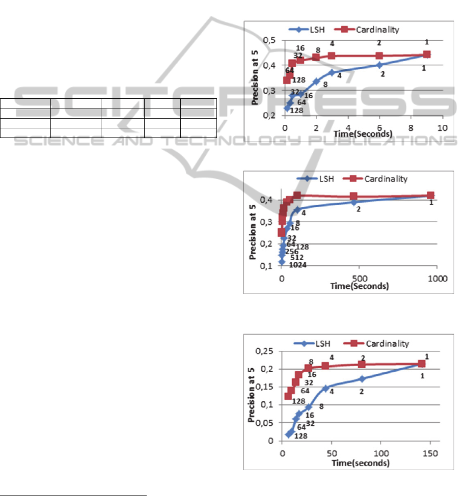
Figures 2, 3 and 4 present precision as a function of

computation time. Each point in a curve represents

the precision of a model with a different predefined

number of clusters. As the number of clusters drops,

more items fall into each cluster, requiring more

computation time. Both methods require the same

amount of time for a given number of clusters, and

split the item set evenly into clusters of identical

sizes.

Figure 2: Performance for the Movie-lens 100k dataset.

Figure 3: Performance for the Movie-lens 1 million

dataset.

Figure 4: Performance for the games dataset.

The clustering time for both methods is

negligible, hence, the overall time is dominated by

FastItem-BasedCollaborativeFiltering

461

the pairwise similarity computations for the larger

clusters. The data points in the curves are average

over 5 repetitions and labelled with the number of

predefined clusters.

5 CONCLUSIONS AND

DISCUSSION

This paper suggests two methods for speeding up the

building of an item-based CF model for top-N

recommendations over implicit datasets. By splitting

items into clusters, and computing pairwise

similarities only for items within the same cluster,

we reduced the computation time dramatically. The

first approach based on LSH and the second on the

cardinality of the item consumption set. Our

experiments show that the cardinality approach

outperformed the LSH, resulting in no decrease in

precision while reducing the computation time up to

10% for the larger dataset.

The cardinality method somehow claims that

similar items also have similar popularity. Although

it might be true and make sense, it is true in our case

only because the similarity function we choose was

Jaccard coefficient which utilized exactly this

aspect. Means that item with low cardinality will

have very small similarity score to item with high

cardinality, if any, because the intersection between

them, the upper part of equation (1), will be close to

zero.

We hence suggest that in order to obtain an

efficient clustering method as pre-process step for

item-base model computation, there has to be some

resemblance between the clustering metric and the

proximity metric used for the items similarity.

Otherwise results may look a bit arbitrary, unless the

clustering method is completely generic as like the

above suggested LSH. For instance applying

content-based clustering such that movies items will

be grouped together according to their Genre may be

a good idea as a clustering method, if the proximity

metric which is used for the item-item similarity

considers the Genres of a movie as part of the

similarity computation. A successful clustering

method will not only be cheap, but also will

encapsulate a hint from the proximity metric which

is later used to calculate the similarity scores. We

therefore suggest that LSH clustering method, which

is not related at all to the similarity metric, is more

recommended if one cannot define a clustering

method which is somehow correlated with the

similarity metric.

An additional benefit of our methods is that the

item-pairs computation of each cluster can be done

in parallel, to further reduce the actual time required

for computing the item-based model.

REFERENCES

J. S. Breese. D. Heckerman, C. Kadie (1998). Empirical

analysis

of predictive algorithms for collaborative

filtering. UAI-98, 43–52.

D. Bridge, J. Kelleher (2002). Experiments in sparsity

reduction: Using clustering in collaborative

recommenders. In Artificial Intelligence and Cognitive

Science (pp. 144-149). Springer Berlin Heidelberg.

S. H. S Chee.(2000) RecTree: A Linear Collaborative

Filtering Algorithm. M.Sc Thesis. Simon Fraser

University.

P. Cremonesi , Y. Koren, R. Turrin (2010). Performance

of recommender algorithms on top-n recommendation

tasks. In Proc. 4th ACM Conference on Recommender

Systems, 39-46.

A. S. Das, M. Datar, A. Garg, S. Rajaram (2007). Google

news personalization: scalable online collaborative

filtering. In Proceedings of the 16th international

conference on World Wide Web (pp. 271-280). ACM.

P. Gionis, P. Indyk, R. Motwani (1999). Similarity search

in high dimensions via hashing. Proceedings of VLDB,

pp. 518–529.

J. L. Herlocker, J. A. Konstan, L. G Terveen, J. T. Riedl

(2004). Evaluating Collaborative Filtering

Recommender Systems. ACM Trans. Information

Systems, vol. 22, no. 1, pp. 5-53, 2004.

P. Jaccard (1901). Étude comparative de la distribution

florale dans une portion des Alpes et des Jura. Bulletin

de la Société Vaudoise des Sciences Naturelles 37:

547–579.

G. Karypis, V. Kumar (1998). A software package for

partitioning unstructured graphs, partitioning meshes,

and computing fill-reducing orderings of sparse

matrices. University of Minnesota, Department of

Computer Science and Engineering, Army HPC

Research Center, Minneapolis, MN.

C. Lin, G. R., Xue, H. J. Zeng, B. Zhang, and Wang, J.

(2014). U.S. Patent No. 8,738,467. Washington, DC:

U.S. Patent and Trademark Office.

G. Linden, B. Smith, J. York (2003). Amazon.com

recommendations: Item-to-item collaborative filtering.

IEEE Internet Computing, 7, 76-80.

B. Sarwar, G. Karypis, J. Konstan, J. Riedl. (2001). Item-

based collaborative filtering recommendation

algorithms. WWW10.

B. M. Sarwar, G. Karypis, J. Konstan, J. Riedl.(2002)

Recommender systems for large-scale e-commerce:

Scalable neighborhood formation using clustering.

In Proceedings of the fifth international conference on

computer and information technology (Vol. 1).

M. O’Connor, J. Herlocker (1999). Clustering items for

collaborative filtering. In Proceedings of the ACM

SIGIR workshop on recommender systems (Vol. 128).

ICAART2015-InternationalConferenceonAgentsandArtificialIntelligence

462

UC Berkeley.

G. Shani, A. Gunawardana (2011). Evaluating

Recommendation Systems. Recommender Systems

Handbook: 257-297.

FastItem-BasedCollaborativeFiltering

463