
The Impact of Demand Correlation on Bullwhip Effect in a
Two-stage Supply Chain with Two Retailers
Jianhua Ji, Huafeng Li, Jie Zhang and Cuicui Meng
Antai College of Economics and Management, Shanghai Jiao Tong University, Shanghai, 200052, China
Keywords: Demand Correlation, Bullwhip Effect, Supply Chain, Supplier, Retailer.
Abstract: In a two-stage supply chain with two retailers, if they have correlated customer demand, forecasting based
on their respective history order might cause significant forecast inaccuracy. Current forecast methods
only use supply chain members’ own history demand information. However, when there are
multi-retailer’s having correlated demand, the common forecasting methods ignore the forecast error
caused by retailers’ interaction. Then, a question comes up that what is the relation between this forecast
error and the bullwhip effect. The present paper studies relation of multi-terminals’ demand correlation
and bullwhip effect in a two-stage supply chain with two retailers. Under centralized or decentralized
information, (1) the impact of retailers’ demand correlation on retailers’/supplier’s bullwhip effect is
studied; (2) the contrast of supplier’s and retailers’ bullwhip effect and the contrast of supplier’s/ retailers’
bullwhip effect under different information sharing condition are studied. The studies show that
multi-terminals’ demand correlation is a cause of supply chain’s bullwhip effect.
1 BACKGROUND
Today, modern supply chain faces more diversified
demands of customers, and more intense horizontal
competition among the parties in the same level of a
supply chain. Especially in a supply chain
producing a homogeneous product, demands of the
parties in the same level undoubtedly get affected
by their interaction. However, this correlation is not
considered in common forecasting methods, such as
moving average, exponential smoothing, or
empirical forecasting. For example, in one
community, there are often more than one
supermarket or convenience store, facing the same
group of customers and providing products same in
price, quality or service. It is obvious that demand
of these terminals should be highly correlated.
When the manager of such retail terminal makes
order based on one of the cited forecast method, if
he or she ignores this correlation, the forecast
inaccuracy would cause a severe inventory backlog
or stock-out.
What is the relationship between retail
terminals’ forecast inaccuracy caused by their
demand correlation and the supply chain’s bullwhip
effect? Or more specifically, what characters of
demand correlation are related to the bullwhip effect?
Under what circumstances (such as centralized
information or decentralized information) may
terminal demand correlation cause bullwhip effect?
Although substantial research has been done on
bullwhip effect in vertical supply chain, not much
research has been performed on bullwhip effect in
supply chain having horizontal competition. In the
present paper we focus on the relation between
demand correlation and bullwhip effect.
2 LITERATURE REVIEW
Lee et al. (1997) prove the existence of bullwhip
effect and describe it with AR (1) demand process.
Later, Lee et al. (2000) prove that bullwhip effect
can be reduced by supply chain information sharing.
Chen et al. (2000a) quantify the bullwhip effect
in a two-echelon supply chain with a single
manufacturer and a single retailer. They examine
the impact of forecasting (moving average
forecasting and exponential forecasting) and order
lead time on the bullwhip effect, and conclude that
bullwhip effect would exist if order lead time is not
zero and that the bullwhip effect would become
304
Ji J., Li H., Zhang J. and Meng C..
The Impact of Demand Correlation on Bullwhip Effect in a Two-stage Supply Chain with Two Retailers.
DOI: 10.5220/0005233003040313
In Proceedings of the International Conference on Operations Research and Enterprise Systems (ICORES-2015), pages 304-313
ISBN: 978-989-758-075-8
Copyright
c
2015 SCITEPRESS (Science and Technology Publications, Lda.)

more severe with larger order lead time. Later, they
extend the conclusion into a multi-stage supply
chain, and reveal that information sharing reduce
but not eliminate the bullwhip effect.
Luong (2007) use a forecasting procedure that
minimizes the expected mean-square forecast error
to estimate the lead time demand, and conclude that
the variance of order will increase with increasing
order lead time. In a later paper, Luong and Phien
(2007) study the bullwhip effect based on a AR(2)
demand process, and extend it into a AR(p) demand
process. They find out that in different ranges of
autoregressive coefficients, the relation between
lead time and bullwhip effect become complicated
that the bullwhip effect does not always exist and
does not always increase when lead-time increases.
Li et al. (2006) research the impact of difference
demand process on the bullwhip effect, and
integrate a general ARIMA (p,d,q) demand process
into the model to analyze the validity of the
production-smoothing model. They find out the
anti-bullwhip effect and the so-called ‘lead-time
paradox’, and they also study the value of
information sharing in supply chain.
3 MODEL DESCRIPTION
Figure 1: One Supplier and Two Retailers Structure.
In the above supply chain with one supplier and two
parallel retailers, there exists demand correlation
between the two suppliers. Here, the concept of
correlation is:
(1) At any period t, retailer 1’s demand
information is determined not only by its own
history demand but retailer 2’s history demand.
(2) At any period t, the random error part of
retailer 1’s demand information is correlated with
that of retailer 2’s. However, the random error part
of retailer 1’s demand information at period t1is
independent with that of retailer 2’s at a different
period t
2
. This assumption is in form of
12
,, ,, 12
,,
(, ) ( ,)
(, )0
it jt jt it
it jt
Cov Cov
Cov
,
(1)
Generally, at the end of period t, the two
retailers place order
,it
O (i=1,2) to the supplier
based on their current respective inventory position.
The supplier will ship the product once it receives
the order. Considering the transportation delay, we
assume that the shipment will arrive at the retailer at
the end of period (t+L), and here constant L means
the same order lead time of the two retailers.
4 DEMAND FORECAST AND
ORDER-UP-TO POLICY
As mentioned in the literature review, forecasting
methods used in most of the previous research on
bullwhip effect include the Moving Average
(MA),the Exponential Smoothing (ES) and the
optimal forecasting method (or Minimum Mean
Square Error forecast, MMSE forecast) (zhang 2004,
Heyman and Sobel 2003, Johnson and Thompson
1975, Chen et al. 2000). In practice, the MA is the
most common forecasting method. The advantage
of this method is that it is easy to use and that it is
good enough to determine the current change of
trend when accuracy is not strictly requested. The
main disadvantage is that the moving averages are
lagging indicators because the method assigns the
same weight rather than greater weight to the more
recent history data, while in practice the more
recent changing trend is more important. The ES is
relatively more suitable in short-to-medium term
forecasting for that it is more sensitive to recent
changing trend. However, it is not that easy to use
because it can be complex to choose a proper
smoothing factor. The optimal forecast method is
the MMSE forecast, which is suitable in
short-to-medium term forecast, sensitive to recent
changing trend, high in forecasting accuracy and the
most complex to use in comparison with other
methods.
We assume that the two retailers use the MMSE
forecast method to estimate the lead time demand.
At the end of period t, history demand sequence of
retail is
,1 ,2 , 1 ,
,
,... ,
i i it it
it
DD D DH
. Through the MMSE
forecast, we can get forecast of demand in next L
periods (here L is the lead
time),
, ,1,2 ,1,
, ... ,
it it it it L it L
FDDD D
, where
conditional expect
10
(,...)
ti
ti t t
D
ED D D D
.
We assume that the two retailers follow
order-up-to inventory policy. Their respective
order-up-to points are determined by lead time
demand forecast at the end of period t. Then we
have
,,1,2 , ,
ˆˆ ˆ
ˆ
...
it it it it L i it
yD D D Z
, where
,
ˆ
it
is
an estimate of the standard variance of retailer i’s
TheImpactofDemandCorrelationonBullwhipEffectinaTwo-stageSupplyChainwithTwoRetailers
305

forecast error during lead time L, and
i
Z
is a
constant measuring retailer i’s service level.
5 MODEL NOTATION
We assume that demand of the two retailers are
correlated, which is a 2-dimension AR(1) process.
1, 1 11 1, 1 12 2, 1 1, 2,
2211,1222,12,
,
ttttt
ttt
da d d d
ad d
(2)
1, 2,
,
tt
are i.i.d. following a distribution with
mean 0, and satisfies
12
2
,,,
,, 12 , ,
() , (, )
(,) , (, )0
it ii it jt
jt it it jt
Var Cov
Cov Cov
(3)
It is obvious that expression (2) becomes two
independent AR(1) processes when
12 21 12
0
.
For the stationary of AR process, we should
choose proper
11 12 21 22
,,,
to make the roots of
11 22 12 21
()()xx
locate in the unit circle.
Let
12
,
denote respectively the mean of the
two retailers’ demand, we have
22 1 12 2
1
11 22 12 21
11 2 21 1
2
11 22 12 21
(1 )
(1 )(1 )
(1 )
(1 )(1 )
aa
aa
(4)
To ensure the positive value of μ
1
and μ
2
, the
following condition should be satisfied:
1 2 22 12 2
11 21 1
0, 0,(1 ) 0,
(1 ) 0
aa a
a
(5)
To simplify expression (1), we
make
,,it it i
zd
, and (1) can be transferred as
1, 11 1, 1 12 2 , 1 1,
2, 21 1, 1 22 2, 1 2,
,
tt tt
tt tt
zz z
zz z
(6)
Denote,
1, 1,
2, 2,
,,
ti ti
ti
ti ti
ti
zy
ZY
zy
1
11 12
21 22
2
1, 1,
2,
2,
2
12
11
2
21
22
,,
,,
()
ti ti
ti ti ti
ti
ti
ti
A
d
DZ
d
Var
(7)
We get the matrix form of (1) as below, where the
characteristic root of A,
1
, or matrix E-A is
invertible.
11
,0
ti ti ti
ZAZ i
(8)
5.1 Bullwhip Effect of the Two
Retailers and the Supplier with
Centralized Demand Information
Centralized demand information means that
retailers share its history demand sequence
,it
H with
each other, so each retailer can forecast and make
order decision based on both retailers’ history
demand.
We substitute
121tL tL tL
ZAZ
for
1tL tL tL
ZAZ
in expression (6), and continue
this iteration to the end:
2
121
12
12 1
...
...
tL tL tL tL tL tL
LL L
tt t tLtL
ZAZ AZ A
AZ A A A
(9)
From
()0
ti
E
, we can have ()
L
tL t
EZ AZ
.
Because for any ARMA process, MMSE forecast of
demand of period t+i equals its conditional
expectation, the MMSE forecasts of
tL
Z
,
1tL
Z
…
1t
Z
are
1
11
,...,
LL
tL t tL t t t
Z
AZ Z A Z Z AZ
(10)
Then, the lead time demand forecast is
11
2
11
()
( ... )
()( )
LL
ti ti
ii
L
t
L
t
DZ
LAA AZ
LEAAAZ
(11)
The lead time demand forecast error is
11
12 2
12
1
()()
( ... ) ( ... )
... ( )
LL
ti ti ti ti
ii
LL L
tt
tL
tL
ZZDZ
AA E A E
AE
(12)
Variance of lead time demand forecast error is
11
12 12 '
22
'
()()
( ... ) ( ... )
( ... ) ( ... )
... ( ) ( ) +
LL
ti ti ti ti
ii
LL LL
LL
Var D D Var Z Z
A
AEAAE
AEAE
AE AE
’
(13)
Denote
1,
2,
t
t
t
o
O
o
as the matrix form of
retailers’ order quantity, and we have
ICORES2015-InternationalConferenceonOperationsResearchandEnterpriseSystems
306

Table 1: Parameter Description.
Parameter Description
1, 2,
,
tt
dd
The demand of Retailer 1,2at period t
1, 2,
,
tt
dd
The demand forecast of Retailer 1, 2 at period t
1, 2,
,
tt
The random variable of demand information faced by Retailer 1, 2 respectively at period t.
Here
2
ii
denote the variance of retailer i’s random variable,and
,
ij ji
denote the correlation of
two retailers’ random variable
,
s
t
The random variable of demand information faced by Supplier, let
,1,2,
s
ttt
11 22
,
The autocorrelation coefficient of Retailer 1, 2
12 21
,
The correlation coefficient describing the correlation between Retailer 1and 2
1, 2,
,
tt
oo
The order quantity of Retail 1, 2 at period t
1, 2,
ˆ
ˆ
,
tt
oo
The forecast order quantity of Retailer 1, 2 at period t
,
s
t
o
The order quantity of Supplier at period t, let
,1,2,
s
ttt
ooo
,
ˆ
s
t
o
The forecast order quantity of Supplier at period t, let
,1,2,
ˆ
ˆˆ
s
ttt
ooo
222
12
,,
s
M
MM
The measure of Bullwhip Effect of Retailer 1, 2 and Supplier
111
1
11
11
1
11
()( )
()( )
LL
tt
LL
tt t ti t
tti
ii
LL
ti t
ti
ii
AZ EA EA
OYY D D D D
ZZZ
(14)
Retailers’ forecast order quantity is
1
1
ˆ
L
tt
OAZ
(15)
Variance of retailers’ order quantity error is
11
ˆ
()(()( ))
L
tt t
Var O O Var E A E A
(16)
Let
11
()( )
L
BEAEA
,and then we have
2
'' '
11 12
2
21 22
ˆ
()()
tt tt
Var O O BE B B B
(17)
Assume that retailers’ order lead time L=1, and
we have
12
11 12
21 22
2
11 12 11 12 11 21
2
21 22 12 22
21 22
1
()( )
1
ˆ
()
11
11
tt
BEAEA EA
Var O O
(18)
Hence, we get the Bullwhip Effect of the two
retailers as the below:
1, 1,
2
1
1,
22 2 2
11 11 12 11 12 12 22
2
11
2, 2,
2
2
2,
22 2 2
22 22 21 22 21 21 11
2
22
ˆ
()
(1 ) 2 (1 )
,
ˆ
()
(1 ) 2 (1 )
tt
t
tt
t
Var O O
M
Var
Var O O
M
Var
(19)
Also, the Bullwhip Effect of the supplier is
s,
s,
2
s,
1, 2,
1, 2,
1, 2,
22
2211 21 11
22
11 22
22 12 22
12
11 21 22 12 12
()
()
()
()
(1 )
(1 ) /
2
2(1 )(1 )
t
t
s
t
tt
tt
tt
Var o o
M
Var
Var o o o o
Var
(20)
5.2 Bullwhip Effect of the Two
Retailers and the Supplier with
Decentralized Demand
Information
Decentralized demand information means that
retailers take each other as competitor and they do
not share information of history demand sequence.
Based on this assumption, each retailer can forecast
and make order decision based on only its own
history demand.
According to expression (6), we have
1, 11 1, 1 12 2, 1 1,
11 1, 1 12 21 1, 2 22 2, 2 2, 1 1,
11 1, 1 12 21 1, 2 12 22 2, 2 12 2, 1 1,
()
tt tt
ttttt
tt ttt
zz z
zzz
zz z
(21)
Now substitute
1, 1 11 1, 2 12 2, 2 1, 1tt tt
zzz
for
2, 2t
z
in the equation above, and we have
1, 11 22 1, 1
12 21 11 22 1, 2
1, 22 1, 1 12 2, 1
()
()
tt
t
tt t
zz
z
(22)
TheImpactofDemandCorrelationonBullwhipEffectinaTwo-stageSupplyChainwithTwoRetailers
307

Following the same procedure, we have
2, 11 22 2, 1
12 21 11 22 2, 2
2, 11 2, 1 21 1, 1
()
()
tt
t
tt t
zz
z
(23)
Let
1 11 22 2 12 21 11 22
,,
,1 ,1
,
it it jj ij
it jt
v
,
equation (22) and (23) become
,1,1 ,2,
2
it it it it
zz zv
(24)
Notice that each retailer only has its own history
demand sequence. From equation (22) and (23),
retailer i can estimate the auto-regression term in
the equation and the auto-correlation part in the
error term, while retailer i cannot estimate the
correlation part in the error term. Hence, neither of
the retailers can forecast the future demand based
on its own history demand sequence.
Lemma 1
Retailer i can use a stable and invertible ARMA
process to model its history demand.
,,
1,1 2,2 ,1
,1,2
it it i
it it it
zz z i
2
2
,, ,
,1
,
,1
() () 4 (, )
2(, )
it it it
it
i
it
it
Var v Var v Cov v v
Cov v v
,
where
1
i
, and the error term satisfies
(1)
,
0
it
E
(2)
'
'
,
,
22 2
,,
()0, ,
() ()/(1 )
it
it
it it i
i
Ett
EVarv
Based on Lemma 1, (22)and(23)become
1, 11,1 21,2 1, 11,1 2,
12, 1 22, 2 2, 2 2, 1
,
tt tttt
tttt
zz z z
zz
,
where
1, 2,
,
tt
are i.i.d.
Assume that retailers’ order lead time L=1, and
we can get the lead time demand forecast and
forecast error as below
,
,, ,
,,,
1,1 2,2 ,1
,,
()
,1,2
it i i
i
it it it
it it it
i
it it it
it it
dz
dd z
Ez H
zz
zi
(25)
Hence, we get the variance of two retailers’
order lead time demand forecast error
,1
,1
2
(),1,2
it
it
i
ddVar i
(26)
Under decentralized information
, retailer i’s
order quantity is
, , ,1 , , ,1 ,
2
,, 12,112,2
1,1 1 ,
()
(1 )
it it it it it it it i
it it i it it
iit i it i
dd zz
z
odz
zz
(27)
Retailers’ forecast order quantity is
2
,
12,112,2
1,1
ˆ
()
it
it it
ii
it
O zz
(28)
Variance of retailers’ order quantity error is
,
,, ,
1
22
,
1
ˆ
ˆ
(1 )
()(1 )
it
it it i it
it i
i
o
o
o
Var o
(29)
Hence, we get the Bullwhip Effect of the two
retailers as below
22
1
,,
2
2
,
(1 )
ˆ
()
i
i
it it
i
it
ii
Var o o
M
Var
(30)
Also, the Bullwhip Effect of the supplier is
s, 1, 2,
s, 1, 2,
2
,1,2,
22 22
11 1 12 2
22
11 22 12
()( )
() ( )
(1 ) (1 )
2
ttt
ttt
s
st t t
Var o o Var o o o o
M
Var Var
(31)
6 BULLWHIP EFFECT
ANALYSIS AND
COMPARISION
In this sector, we analyze the impact of demand
correlation on retailer and supplier Bullwhip Effect.
To eliminate the possible influence of other
parameters, we assume that
11 22 12 21 11 22
===
,,
. This assumption is
reasonable in practice, because in the same local
market there are often two retailers similar in both
market share and products sold.
6.1 Numerical Analysis of
2
i
M
under
Centralized Information
With conditions of centralized information, L=1,
and MMSE forecasting, the two retailers face
bullwhip effect as below
ICORES2015-InternationalConferenceonOperationsResearchandEnterpriseSystems
308
1,
1,
2
1
1,
22 2 2
11 11 12 11 12 12 22
2
11
2,
2,
2
2
2,
22 2 2
22 22 21 22 12 21 11
2
22
()
(1 ) 2 (1 )
()
(1 ) 2 (1 )
t
t
t
t
t
t
Var o o
M
Var
Var o o
M
Var
(32)
When
11 22 12 21 11 22
===
,,
, we
get
2
1
M
=
2
2
M
.
Then, it is obvious that
2
2
22
2
2
2(1 ) 2
,
2(1 )
,, ,12
ii ij jj
i
ij
ij ii ii
iii
ij
ij ii
dM
d
dM
i j and i j or
d
(33)
Let
2
0
i
ij
dM
d
,we get
2
(1 )
ij ii
ij
jj
。
From
1, 1
ii ij
,we get
01 2
ii
, so
2
/
iij
dM d
and
ij
have the same sign.
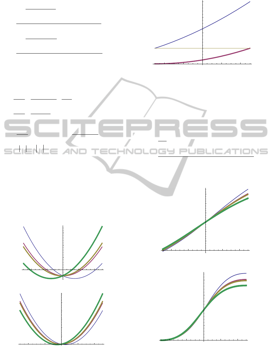
Figure 2, Figure 3 and Figure 4 display the
relation between Bullwhip Effect and demand
correlation under centralized information.
Let
11 22 11
10, 0.5, 0.5
. Notice that to
ensure the stability, let
12
0.5,0.5
(- )
.
2
1
M
varies
with
12
as shown in Figure2.
Let
11 22 11 22
10, 0.5, 0.5
. To ensure
the stability,
12
(0.5,0.5)
.
2
s
M
varies with
ij
as
shown in Figure3.
0.4
0.2 0.2 0.4
2.4
2.5
2.6
11
=0.5
,
12
= -10,-1,1,10
(thin->thick)
2
1
M
12
0.4
0.2 0.2 0.4
0.30
0.35
0.40
0.45
0.50
0.55
11
= -0.5
,
12
= -10,-1,1,10
(thin->thick)
12
2
1
M
Figure 2: Retailer’s Bullwhip Effect under Centralized
demand information.
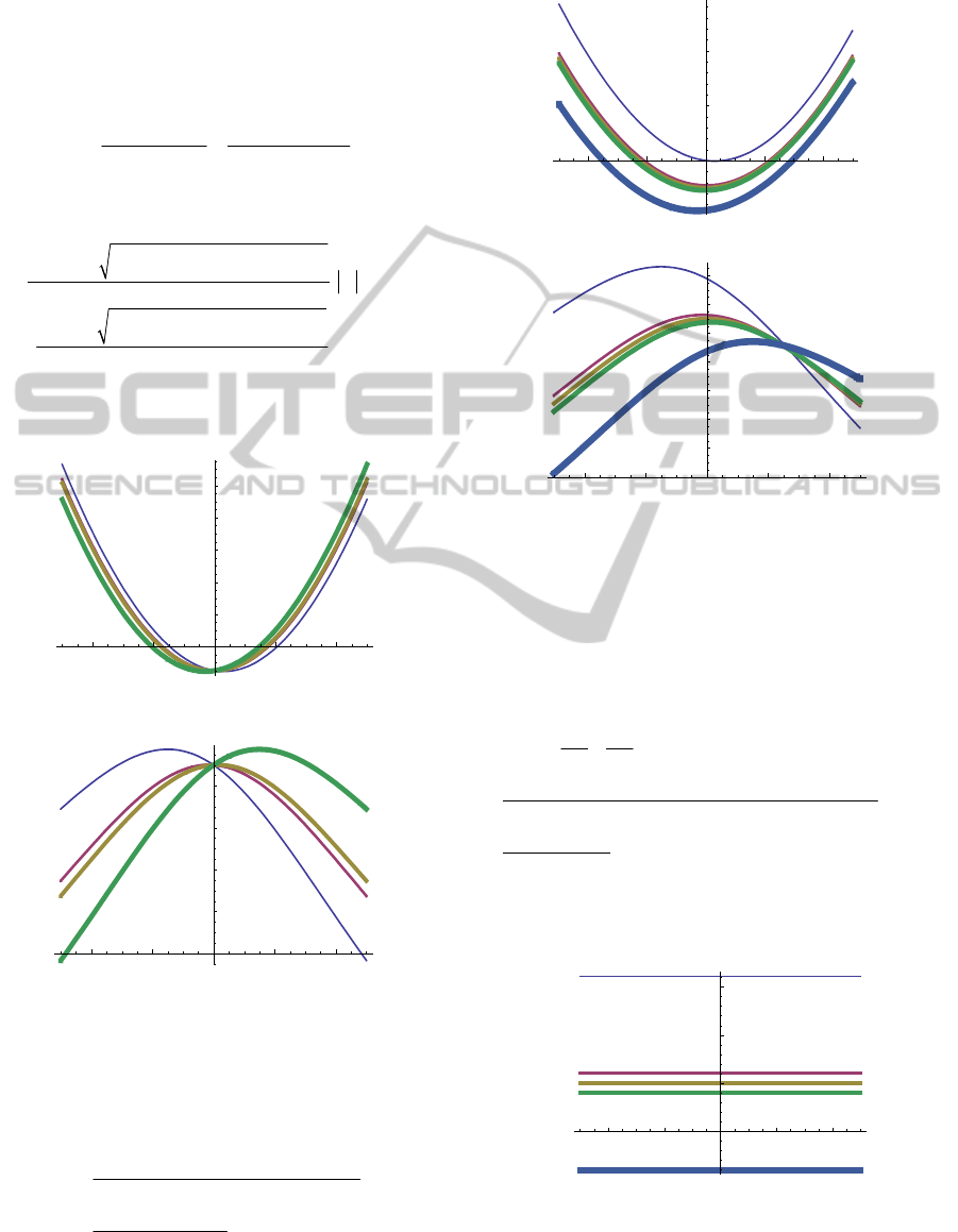
0.4
0.2 0.2 0.4
1
2
3
4
11 22
=0.5,0.5
(thin->thick)
2
s
M
12
Figure 3: Supplier’s Bullwhip Effect under Centralized
demand information.
Next, compare the retailers’ bullwhip effect with
the supplier’s under centralized demand information,
when
11 22 12 21 11 22
===
,,
:
2
1
2
2
12 22
22 2 2 2
11 11 12 11 12 12 22 11
1
[(1 ) 2 (1 ) ] /
s
i
M
Ratio
M
(34)
Let
11 22 11 22
10, 0.5, 0.5
,
1
Ratio
varies with
12
as shown in Figure 4.
0.4
0.2 0.2 0.4
0.6
0.8
1.0
1.2
1.4
1.6
11
=0.5
,
12
=-10,-1,1,10
(thin->thick)
12
Ration
1
0.4
0.2 0.2 0.4
0.5
1.0
1.5
2.0
11
=-0.5
,
12
=-10,-1,1,10
(thin->thick)
12
Ration
1
Figure 4: Bullwhip Effect Contrast under Centralized
demand information.
TheImpactofDemandCorrelationonBullwhipEffectinaTwo-stageSupplyChainwithTwoRetailers
309
6.2 Numerical Analysis of
2
i
M
under
Decentralized Information
With conditions of decentralized information, L=1,
and MMSE forecasting, the two retailers face
bullwhip effect as below
22
,
1
,
2
2
,
(1 )
()
it
ii
it
i
it ii
Var o o
M
Var
(35)
where
11122
22
,, ,,1
,,1
22
,, ,,1
2
() () 4 (, )
,1
2(, )
() () 4 (, )
2
it it it it
ii
it it
it it it it
i
Vv Vv Covv v
Cov v v
Vv Vv Covv v
(36)
When
11 22 11 22
10, 0.5, 0.5
,
2
1
M
varies with
12
as shown in Figure 5.
0.4
0.2 0.2 0.4
2.6
2.8
3.0
3.2
3.4
11
=0.5
,
12
=-10,-1,1,10
(thin->thick)
2
1
M
12
0.4
0.2 0.2 0.4
0.18
0.20
0.22
0.24
11
=-0.5
,
12
=-10,-1,1,10
(thin->thick)
2
1
M
12
Figure 5: Retailer’s Bullwhip Effect under Decentralized
demand information.
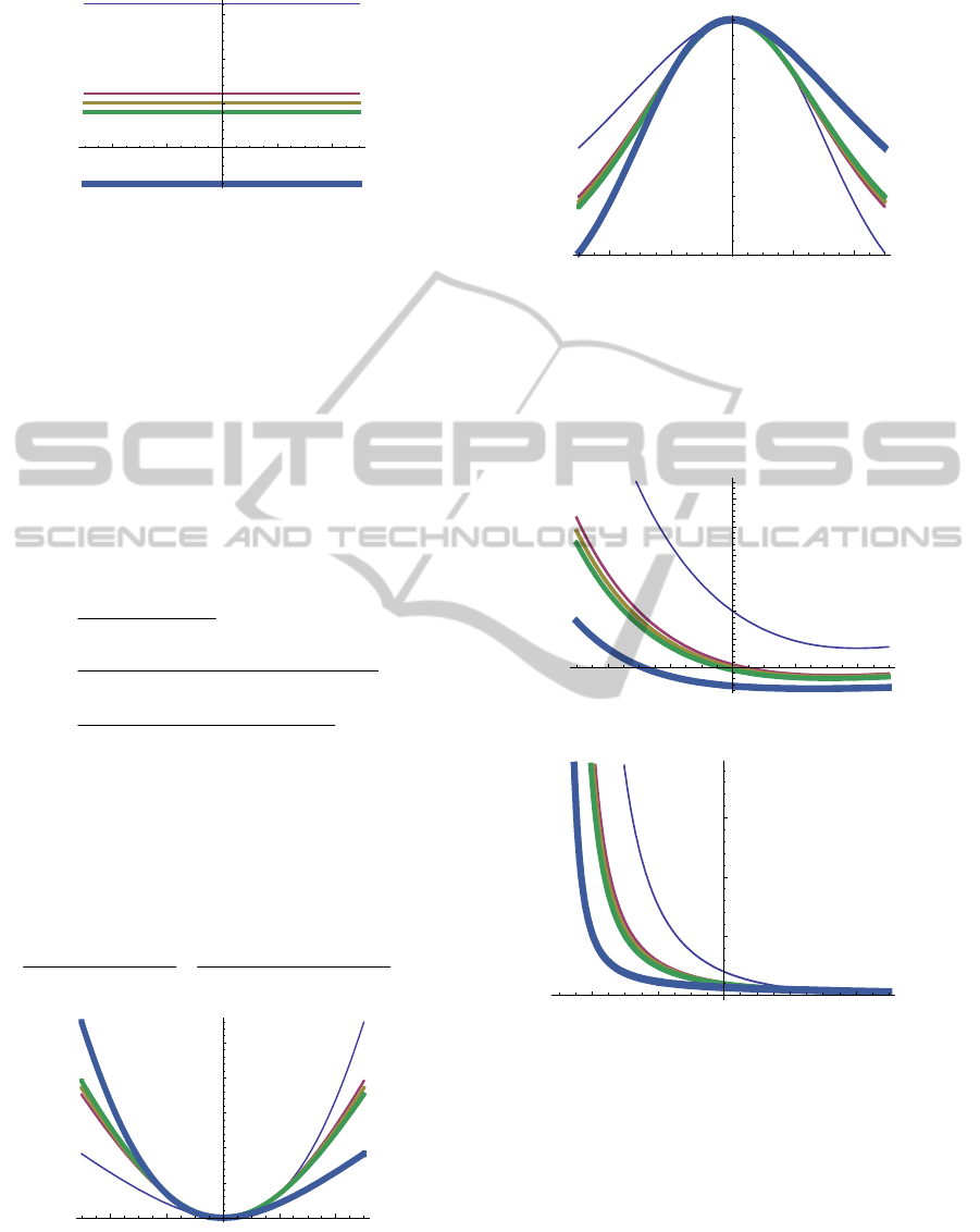
Under decentralized information, bullwhip
effect of the supplier is
22 22
11 1 1 2 2
2
22
11 22 12
22
11 1
22
11 22 12
(1 ) (1 )
2
2(1 )
2
s
M
(37)
When
11 22 11 22 12 21
10, 0.5, 0.5,
,
2
s
M
varies with
ij
as shown in Figure 6.
0.4
0.2 0.2 0.4
3.0
3.5
11
=0.5
,
12
=-10,-1,0,1,10
(thin->thick)
2
s
M
12
0.4
0.2 0.0 0.2 0.4
0.16
0.18
0.20
0.22
0.24
0.26
0.28
11
=-0.5
,
12
=-10,-1,0,1,10
(thin->thick)
2
s
M
12
Figure 6: Supplier’s Bullwhip Effect under Decentralized
demand information.
Under decentralized information,
if
11 22 12 21 11 22
===
,,
, we have
22
12
=
M
M .Now
we compare the retailers’ bullwhip effect with the
supplier’s.
22
2
22
1
22 22 2 2
1 1 1 1 2 2 11 22 12
22 2
11 1 11
2
11
22
11 22 12
n
[(1 ) (1 ) ] / ( 2 )
[(1 ) ] /
2
2
ss
i
MM
Ratio
MM
(38)
When
11 22 11 22 12 21
10, 0.5, 0.5,
,
2
nRatio
varies with
ij
as shown in Figure 7.
0.4
0.2 0.2 0.4
1.00
1.05
1.10
11
=0.5
,
12
=-10,-1,0,1,10
(thin->thick)
2
R
ation
12
Figure 7: Bullwhip Effect Contrast under Decentralized
demand information.
ICORES2015-InternationalConferenceonOperationsResearchandEnterpriseSystems
310
0.4
0.2 0.2 0.4
1.00
1.05
1.10
11
=-0.5
,
12
=-10,-1,0,1,10
(thin->thick)
2Ration
12
Figure 7: Bullwhip Effect Contrast under Decentralized
demand information (cont.).
6.3 Bullwhip Effect Contrast between
Centralized and Decentralized
Demand Information
In this section, we analyze the retailers’/supplier’s
bullwhip effect contrast between centralized and
decentralized information.
Let Ri represent the ratio of retailer i’s bullwhip
effect under centralized information to that under
decentralized information
2
2
22 2
1
22 22 2
22
1
22 22
()
()
[(1 ) ] /
[(1 ) 2 (1 ) ] /
(1 )
(1 ) 2 (1 )
i
i
i
ii ii
ii ii ij ii ij ij jj ii
ii
ii ii ij ii ij ij jj
M decentralized
R
M centralized
(39)
When
11 22 11 22 12 21
10, 0.5, 0.5,
,
we get
12
RR
, and
1
R
varies with
12
as shown
in Figure 8.
Let S represent the ratio of supplier’s bullwhip
effect under centralized information to that under
decentralized information
22
2
11 1
222
11 21 11 12
(1 )
()
()(1)()
s
s
M decentralized
S
M centralized
(40)
0.4
0.2 0.2 0.4
1.1
1.2
1.3
1.4
1.5
11
=0.5
,
12
=-50,-5,0,5,50
(thin->thick)
1
R
12
Figure 8: Retailer’s B.E. Contrast Between Centralized
And Decentralized D-I.
0.4
0.2 0.2 0.4
0.4
0.6
0.8
1.0
11
=-0.5
,
12
=-50,-5,0,5,50
(thin->thick)
12
1
R
Figure 8: Retailer’s B.E. Contrast Between Centralized
And Decentralized D-I (cont.).
When
11 22 11 22 12 21
10, 0.5, 0.5,
,
S varies with
ij
as shown in Figure 9.
0.4
0.2 0.2 0.4
1.5
2.0
2.5
3.0
3.5
4.0
11
=0.5
,
12
=-50,-5,0,5,50
(thin->thick)
12
S
0.4
0.2 0.2 0.4
5
10
15
11
=-0.5
,
12
=-50,-5,0,5,50
(thin->thick)
12
S
Figure 9: Supplier’s B.E. Contrast Between Centralized
And Decentralized D-I.
7 CONCLUSIONS AND
INSIGHTS
7.1 Main Conclusions
(1) Under decentralized information, when
ii
>0:
TheImpactofDemandCorrelationonBullwhipEffectinaTwo-stageSupplyChainwithTwoRetailers
311

2
i
M
,
2
s
M
is monotone increasing as absolute
value of
12
increases.
2
ationR
varies around 1, and its monotone
decreasing as
12
increases is not significant. This
situation indicates that
12
is not strongly related to
the amplification of bullwhip effect going up the
supply chain.
12
has little impact on bullwhip
effect.
(2) Under centralized information, when
ii
>0:
Bullwhip effect of retailer/supplier is monotone
increasing as
12
increases, and the amplification is
significant.
When
12
>0,
1
ationR
2
centr s
M /
2
centr i
M >1,and
1
ationR
is monotone increasing as
12
increases. It
means that the amplification of variance of order in
supplier stage is larger than that in retailer stage,
and this difference increases with the value of
12
.
This situation indicates that larger
12
will increase
the amplification of variance of order quantity
spreading to the upstream supply chain.
When
12
<0,
1
ationR
<1 , and
1
ationR
is
monotone increasing as
12
increases. It means
that the amplification of variance of order in
supplier stage is smaller than that in retailer stage,
and this difference decreases as
12
increases. The
impact of number of stages of supply chain on
bullwhip effect is not effected by
12
.
ij
has little impact on bullwhip effect.
(3) When
ii
<0,
12
and
12
both have little
impact on bullwhip effect.
7.2 Management Insights
To sum up, what we should pay attention to are as
following:
(1) When retailers’ demands are positive
correlated, no matter under centralized or
decentralized information, this correlation has
significant impact on retailers’/supplier’s bullwhip
effect.
(2) Under decentralized information, both
retailers’ and supplier’s bullwhip effect increases as
the absolute value of retailers’ demand correlation
increases, and bullwhip effect in supplier stage and
retailer stage are almost the same.
(3) Under centralized information, when
retailers’ demands are positive correlated, both
retailers’ and supplier’s bullwhip effect increases as
retailers’ demand correlation increases, and
bullwhip effect level in supplier stage is larger than
that in retailer level. It indicates that under
centralized information the impact of number of
supply chain stages on bullwhip effect is related
with the retailers’ demand correlation.
(4) Under centralized information, when and
only when retailers’ demands are negative
correlated (
0
ij
), the supplier’s bullwhip effect
will be less than retailers’. It indicates that under
centralized information supplier’s demand forecast
become more accurate as the result of retailers’
competition.
Hence, when retailers’ demands are correlated,
besides the well-known causes of bullwhip effect
(such as lead time, number of supply chain stages),
any member in the supply chain should consider the
impact of multi-terminals’ demand correlation on
bullwhip effect when making production plan.
Furthermore, under centralized information, when
retailers’ demand are positive correlated, the
bullwhip effect in supplier stage is higher than that
in retailers’ stage; on the contrary, under centralized
information, when retailers’ demand are negative
correlated, the bullwhip effect in supplier stage is
lower than that in retailers’ stage. These conclusions
provide theoretical reference about bullwhip caused
by terminals’ demand correlation for enterprises to
make production plan.
ACKNOWLEDGMENTS
This research is supported in part by National
Science Foundation of China Grants (70732003).
REFERENCES
Chen, F., Drezner, Z., Ryan, J.K., and Simchi-Levi,
D. (2000a), ‘Quantifying the bullwhip effect in a
simple supply chain’
, Management Science, 46 ,
436–443.
Chen, F., Ryan, J.K., and Simchi –Levi, D. (2000),
‘The impact of exponential smoothing forecasts
on the bullwhip effect’,
Naval Research
Logistics
, 47, 269–286.
Heyman, D.P. and Sobel, M.J. (2003), Stochastic
Models in Operations Research: Stochastic
Optimization (Vol.2),
New York: Courier Dover
Publications.
Johnson, G.D. and Thompson, H.E. (1975),
Optimality of myopic inventory policies for
certain dependent demand processes,
Management Science, 21, 1303–1307.
ICORES2015-InternationalConferenceonOperationsResearchandEnterpriseSystems
312

Lee H.L, Padmanabhan V. and Whang S. (1997),
Information Distortion in a Supply Chain: The
Bullwhip Effect,
Management Science, 43,
546-558.
Lee, H.L ,So K.C. and Tang, C.S. (2000), The value
of information sharing in a two-level supply
chain,
Management Science, 46, 626-643.
Li, G., Wang, S.Y. and Yu, G. (2006), A study on
bullwhip effect and information sharing in
supply chains,
Changsha: Hunan University
Press
. (in Chinese).
Luong, H.T. (2007), Measure of Bullwhip Effect in
Supply Chains With Autoregressive Demand
Process,
European Journal of Operational
Research
, 180, 1086-1097.
Luong, H.T. and Phien, N.H. (2007), Measure of
Bullwhip Effect in Supply Chains—The case of
high order Autoregressive Demand Process,
European Journal of Operational Research, 183,
197-209.
Zhang, X.L. (2004), The impact of forecasting
methods on the bullwhip effect,
International
Journal of Production Economics
, 88, 15-27.
TheImpactofDemandCorrelationonBullwhipEffectinaTwo-stageSupplyChainwithTwoRetailers
313
