
Temporal Selection of Images for a Fast Algorithm for Depth-map
Extraction in Multi-baseline Configurations
Dimitri Bulatov
Fraunhofer Institute of Optronics, System Technologies and Image Exploitation
Gutleuthausstr. 1, 76275 Ettlingen, Germany
Keywords:
Aggregation Function, Interaction Set, Depth map, Plane Sweep, Triangle Mesh.
Abstract:
Obtaining accurate depth maps from multi-view configurations is an essential component for dense scene
reconstruction from images and videos. In the first part of this paper, a plane sweep algorithm for sampling
an energy function for every depth label and a dense set of points is presented. The distinctive features of this
algorithm are 1) that despite a flexible model choice for the underlying geometry and radiometry, the energy
function is performed by merely image operations instead of pixel-wise computations, and 2) that it can be
easily manipulated by different terms, such as triangle-based smoothing term, or post-processed by one of the
numerous state-of-the-art non-local energy minimization algorithms. The second contribution of this paper is
a search for optimal ways to aggregate multiple observations in order to make the cost function more robust
near the image border and in occlusions areas. Experiments with different data sets show the relevance of the
proposed research, emphasize the potential of the algorithm, and provide ideas of future work.
1 INTRODUCTION
Using multiple images in order to extract high qual-
ity depth maps has become extremely popular in the
recent years (Goesele et al., 2007), especially for the
application of 3D urban terrain reconstruction from
aerial and even UAV-borne imagery (Rothermel et al.,
2014). Even though pixels in homogeneously tex-
tured areas of images cannot be reliably matched
without exploiting assumptions on the geometry of
the scene, such as piecewise smoothness assumption,
the advantages in comparison with binocular methods
in areas of repetitive texture, occlusions, and moving
objects are evident and well-known. These advan-
tages are explained by multiple observations that can
resolve ambiguities both near repetitive texture pat-
terns and occlusions.
There is much work done in exploring the influ-
ence of different algorithm parameters that are valid
for both binocular and multi-view configurations,
such as window size (Nakamura et al., 1996; Boykov
et al., 1998; Kang et al., 2001), data cost function for
measuring radiometric deviations (Hirschm¨uller and
Scharstein, 2009), or smoothness parameters for non-
local optimization algorithms (Hansen and O’Leary,
1993; Kolmogorov, 2003). However, only a few re-
lated works perform detailed analysis about the nu-
merous ways to consider these multiple observations.
This is where our particular interest about the aggre-
gation function comes from. Note that many authors
also use this term in the binocular configuration. They
refer to the way to sum up costs from neighboring pix-
els, where neighborhood relations can be given by a
geometric adjacency, segmentation results of images,
etc. In this paper, the term aggregation will always
refer to the multiple observations of a multi-baseline
configuration. The local neighborhoods of pixels can
be considered for all images at once or for pairs of
images. The parameter regulating which pairs should
be considered is called, according to (Kolmogorov,
2003), interaction set and is the second important pa-
rameter concerning merely multi-baseline configura-
tions. From the related work (Kang et al., 2001) we
know that the temporalselection of images is a crucial
idea to reduce the number of mismatches near occlu-
sions, but we noticed that many authors (Nakamura
et al., 1996; Kang et al., 2001; Okutomi and Kanade,
1993) consider only the data cost functions based on
Sum of Squared Differences (SSD) for the perfor-
mance analysis. However, for configurations with
strong deviations of luminance between images, other
cost functions should be applied. It will be shown that
the best choices of the interaction set and the aggrega-
tion depends both on the geometric configurations of
395
Bulatov D..
Temporal Selection of Images for a Fast Algorithm for Depth-map Extraction in Multi-baseline Configurations.
DOI: 10.5220/0005239503950402
In Proceedings of the 10th International Conference on Computer Vision Theory and Applications (VISAPP-2015), pages 395-402
ISBN: 978-989-758-091-8
Copyright
c
2015 SCITEPRESS (Science and Technology Publications, Lda.)

cameras and the measure for radiometric deviations.
It is important to emphasize that we do not pur-
sue an evaluation of the related approaches; first, be-
cause for many approaches – including our work –
the factor of speed is very important, and second, be-
cause there are many ways to compensate for outliers
in single depths maps, for example, by means of depth
maps fusion (Pollefeys et al., 2008) or corresponding
linking (Koch et al., 1998) within the state-of-the-art
multi-view systems for surface reconstruction (Goe-
sele et al., 2007). Because of this reason, we will not
perform a detailed study of all steps that somehow can
influence the results of different choices of previously
mentioned parameters. These steps include the spatial
techniques, such as variable windows, see (Nakamura
et al., 1996; Kang et al., 2001) (because they usu-
ally make slower the plane-sweeping approach and
have been sufficiently investigated in binocular con-
figurations) as well as the triangle-based smoothing
proposed in (Bulatov et al., 2011). However, we
give a short description of the modules for non-local
optimization on 2D Markov Random Fields meth-
ods while presenting our procedure for multi-baseline
depth map computation. This will be done in Sec.2
in order to illustrate the concept of our fast, modular
plane-sweep algorithm. The main study on different
interaction sets and aggregation functions is presented
in Sec.3. The results for a benchmark sequence, the
well-known Tsukuba data set, and several sequences
of aerial video frames are described in Sec. 4 while
main conclusions and ideas of future research com-
plete our work in Sec.5.
2 OUR MULTI-BASELINE PLANE
SWEEP ALGORITHM
The input of our algorithm consists of several (5 to
10) images J
0
,...,J
K
,K > 1 as well as corresponding
projection matrices P
0
,...,P
K
. The desired output is
assigning a scalar depth value to every pixel of a ref-
erence frame J
r
; this reference frame can be one of the
input images, possibly in the middle of the sequence,
or a virtual image, at an arbitrary position. As in many
algorithms for depth maps extraction (Hirschm¨uller,
2008; Scharstein and Szeliski, 2002), we identify two
main steps: Multi-baseline data cost aggregation and
non-local optimization.
For all pixels i of the reference image and any
discretized depth value d(s),s = 1,2,...,S, the data-
driven energy term E
data
(s) should be summed up
over the input images. The task is to project pix-
els from image to image by homographies induced
by planes parallel to the reference image plane at dis-
tance d(s). However,instead of pixel-wise projection,
a standard plane-sweep algorithm presupposes warp-
ing the image J
k
by the homography H
k
(s):
H
k
(s) = M
k
+ [0
3
0
3
e
k
/d], where (1)
M
k
= P
{4}
r
P
{4}
k
−1
and e
k
= P
r
kern(P
k
)
are the infinite homography and the epipole, respec-
tively. We denote by P
r
the reference camera, given
by a 3 × 4 matrix, and P
{4}
represents the first three
columns of P. All variables in (1) are homogeneous
quantities, but they are normalized. Camera matrices
are scaled the way that the norm of the third row of
P
{4}
is 1, the objects in the foreground have positive
depth values, and the camera center kern(P), which
is the one-dimensional null-space of P, must have the
fourth homogeneous coordinate 1. The proof of (1) is
given in e.g. (Bulatov et al., 2011). We denote the im-
age J
k
warped by H
k
(s) into the coordinate system of
the reference frame by J
k
(s). The advantage to warp
the images instead of taking a loop over pixels is that
many programming languages are optimized for op-
erations with images and matrices; these operations
and those to come can be efficiently implemented.
Indeed, most cost function of the cost functions
considered in (Hirschm¨uller and Scharstein, 2009)
can also be performed simultaneously over images.
For example, the well-known truncated SAD (Sum of
Absolute Differences) cost function is equivalent to
the convolution of the difference image
C
data
(s,k,k
′
) = min(g|J
k
(s) − J
k
′
(s)|
∗ f
,1) (2)
with g a normalization scalar and f a kernel filled
by ones and having the size of the correlation mask.
The SSD function can be formulated in an analogous
way. After trivial simplifications, the NCC (Normal-
ized Cross Correlation) function is formulated as
c =
(J
k
J
k
′
)
∗ f
− (J
k
)
∗ f
(J
k
′
)
∗ f
r
(J
2
k
)
∗ f
− (J
k
)
2
∗ f
(J
2
k
′
)
∗ f
− (J
k
′
)
2
∗ f
, (3)
and C
data
(s,k,k
′
) = (1− c)/2. In (3), J
k
= J
k
(s),J
k
′
=
J
k
′
(s) and all products are taken element-wise. Also,
two important non-parametric cost functions intro-
duced in (Hirschm¨uller and Scharstein, 2009), Mu-
tual information and Census, can be formulated in an
analogous way, as
C
data
= M (J
k
(s),J
k
′
(s))
∗ f
and
C
data
=
1
N
∑
N
n=1
D
n
k
(s) 6= D
n
k
′
(s)
∗ f
,
(4)
respectively. Here, f is an optional correlation mask,
M (·,·) are the rows and the columns of the mutual
information table and D are the entries of the N-bits
VISAPP2015-InternationalConferenceonComputerVisionTheoryandApplications
396

descriptor of J
k
(s) which is coded as an N-bit image.
Given that the underlying model of radiometry trans-
formation is correct, one common thing about equa-
tions (2)-(4) is that for all pixels for which the cor-
responding 3D point is situated near the plane num-
ber s, and it is visible in images J
k
,J
k
′
, the values of
C
data
(s,k,k
′
) are supposed to be relatively low. The
task of the next section is to find fast ways to aggre-
gateC
data
(s,k,k
′
) into E
data
(s) such that border pixels
and occluded pixels are treated in a robust way.
For now, however, we assume E
data
(s) as input,
which was collected over all values of S. It is possi-
ble to add the triangle-based energy term calculated
by means of some points with already available depth
values, as proposed in (Bulatov et al., 2011), but again
in form of an image
E
mesh
(s) = a
T
W
T
min(|s− S
T
|,s
0
), (5)
where S
T
is the map of labels induced by the trian-
gular interpolation of depth values from the already
available 3D points, W
T
(i) is the weight how close
the pixel i is to a vertex of the mesh, a
T
is the a-priori
probability that a triangle is consistent with the sur-
face, and s
0
is a scalar. Alternatively or additionally,
it can be subject to a non-local optimization with one
of the state-of-the-art algorithms. The goal of such
an algorithm is to find a strong local minimum of the
energy function:
E(s) =
∑
i
E
local
(s
i
)
|
{z }
E
data
(s
i
)+E
mesh
(s
i
)
+
∑
i, j∈N
E
smooth
(s
i
,s
j
), (6)
where N is the 4-neighborhood between pixels, and
E
smooth
is usually the truncated linear penalty term
1
.
Many algorithms for non-local optimization are an-
alyzed by (Szeliski et al., 2006) for depth map ex-
traction and for many other problems of Computer
Vision. In what follows, a short overview of seven
algorithms integrated into our pipeline will be given.
1 Our default method is semi-global optimization.
As described in (Hirschm¨uller, 2008), the main
idea is to sum up costs along 4, 8, or 16 paths by
means of a recursive function thus allowing an ap-
proximationof E(S) from (6) as a H ×W ×S array
so that the output is given by minimizing this ma-
trix along the third dimension. H,W are the height
and width of the reference images, respectively.
2 Dynamic programming is a special case of the pre-
vious method with only one path and, as a conse-
quence, a slightly more efficient implementation.
1
For the sake of computational resources, the matrix
representing the local energy term in (6) is usually rescaled
to integer numbers, but in Sec. 3, they will be in range [0; 1].
We implemented the method proposed by (Bel-
humeur, 1996).
3 The method of alpha-expansions based on graph-
cuts can solve (6) in a polynomialtime for the case
that s is a binary variable (see e.g. (Kolmogorov,
2003)). The labels are set in a random order. For
every label α, an alpha-expansion overwrites the
labels of some pixels with this value α. An outer
loop repeats the S expansions for several times.
4 A similar approach, known as alpha-beta-swap,
presupposes swapping labels of pixels within an
inner iteration. Similarly to alpha-expansions, we
used the implementation of (Delong et al., 2012)
designed for arbitrary data function on Markov
Random Fields with a metric smoothness func-
tion.
5 The Tree Re-Weighted Sequential method, TRW-
S, (Kolmogorov, 2006) is a modification of the
method of (Wainwright et al., 2005) and allows
manipulation of the local energy term of (6) ac-
cording to a convex combination of trees and in
the way that the smoothness term vanishes. A tree
is a graph without loops for which many fast op-
timization methods exist and the global minimum
can be obtained. Thus, the distinctive feature of
the TRW-S method is that a lower bound for the
global minimum of (6) is available.
6 Without convex combination of trees, a standard
belief propagation algorithm, see e.g.(Sun et al.,
2003), is also implemented by (Kolmogorov,
2006). It is faster than the TRW-S method, how-
ever, usually at costs of computational results.
7 Finally, a modification of the filtering methodpro-
posed by (Pollefeys et al., 2008) allows determin-
ing the lower cost value for the entire image given
that the labels of its neighbors are fixed. Formally,
for a label s, we consider the term
ˆ
E(s) = E
local
(s) + λmin(|s− S
0
|,s
0
)
∗ f
, (7)
where S
0
is the initialization of the depth map (for
example, the minimizer of the local energy term
in (6)), f is a correlation mask with zero in the
center, s
0
is a scalar, and λ is a constant, which
can be multiplied by a confidence matrix, for ex-
ample, the one proposed in Eq. (28) of (Pollefeys
et al., 2008). The minimum-taking along the third
dimension of
ˆ
E (7) yields a new labeling
ˆ
S
0
. Ex-
periments with replacing S
0
by
ˆ
S
0
, the local term
in (7) by
ˆ
E, and performing the convolution sev-
eral times are currently being carried out.
TemporalSelectionofImagesforaFastAlgorithmforDepth-mapExtractioninMulti-baselineConfigurations
397

3 CHOICE OF AGGREGATION
FUNCTION AND
INTERACTION SET
In this section, we are interested about how to aggre-
gate information from single data cost functions C =
C
data
(s,k,k
′
) into a data cost energy term E
data
(s).
Equations (2)-(4) handle pairs of images and the three
arising questions are: Which pairs should be consid-
ered? How should they be aggregated? Is it necessary
to aggregate pairs or a simultaneous treatment of im-
ages can be carried out as well? Sec.3.1 is dedicated
to choosing pairs of images while Sec.3.2 elaborates
several aggregation functions.
3.1 Choice of Interaction Set
There are K(K + 1)/2 possible pairs of interactions.
As a consequence, a subset must be selected if we
want our algorithm to be linear in the number of
views. One possibility (Type I1) is to consider the
cost terms between the reference image J
r
and other
images, see (Pollefeys et al., 2008; Bulatov et al.,
2011). Another choice, namely to use neighboring
images, is proposed in (Kolmogorov, 2003). We de-
note it by Type I2 for our evaluation section. The ad-
vantages of this latter choice is that the images are
treated symmetrically which helps to avoid errors re-
sulting from radiometric irregularities in the reference
image (reflections, dead pixels in infrared images,
etc.). The disadvantage is that in many situations, the
neighboring images look very similar and so we must
live with a shorter baseline and consequently, a lower
depth accuracy that theoretically can be obtained.
In addition to these two types of interaction sets,
we also consider the union of I1 and I2. If the num-
ber of images is low or if a higher computation cost is
not a problem, it is also possible to consider all pairs
of images to obtain the highest possible redundancy.
These types of interaction sets are denoted by I3 and
I4, respectively. It must also be mentioned that con-
sideration of different interaction sets only takes place
in case of pairwise evaluations of data cost functions.
However, data cost aggregation may be carried out in
a different way as pairwise evaluation. Hence, we will
present an example of a non-pairwise aggregation in
the next section.
3.2 Choice of Aggregation Function
We start by treating pairwise computed single data
cost functions C(s,k,k
′
) where <k,k
′
> belong to the
interaction set. An obvious idea (Type A1) to consider
the (weighted) average of all cost values
E
data
(s) = 1/N
∑
<k,k
′
>
w(k,k
′
)C(s,k,k
′
), (8)
where N =
∑
<k,k
′
>
w(k,k
′
) is the number of interac-
tions, probably achieves its best impact if there are
only a few images. This strategy was followed by
(Zhang et al., 2003; Heinrichs et al., 2007) for trinoc-
ularly rectified triplets of images. The latter approach
only uses the interaction set of Type I1 and does not
consider the cost computation between the remaining
pair of images. The weights w(k,k
′
) are set to 1.
However, for an increasing number of images,
strategies of discarding gross errors should be applied.
Optimally, this can be done by selecting only the best
cost values, as in (Bulatov et al., 2011; Irschara et al.,
2012; Furukawa and Ponce, 2010). We denote by
c
max
the maximum correlation coefficient and by G
the subset of the interaction set where the single data
cost function does not exceed c
max
, that is, radiomet-
rically consistent pairs of images. Furthermore,
ˆ
k is
the minimum number of radiometrically consistent
pairs of images and
ˆ
K(s) denotes the cardinality of
G. Then, the aggregation function of Type A2 from
(Bulatov et al., 2011) is
E
data
(s) =
1
a
ˆ
K(s) + b
∑
<k,k
′
>∈G
C(s,k,k
′
), (9)
if
ˆ
K(s) >
ˆ
k and 1 (the maximum value) otherwise.
Note that
ˆ
K(s) is itself an image of the same size as
J . Thus, the division is element-wise. The scalar pa-
rameters a and b are supposed to encourage the pixels
to be visible in the large number of views. We choose
a = 1+ ε, b = −ε
ˆ
k and ε > 0. This means that the
value of (9) coincides with that of (8) when
ˆ
K =
ˆ
k
and it is slightly smaller when
ˆ
K >
ˆ
k. Moreover, we
denote by Type A3 the aggregation function proposed
by (Irschara et al., 2012), which is the truncated ver-
sion of (8).
The idea of the time-optimized software for video-
processing of (Pollefeys et al., 2008) was to reduce
the influence of occlusions by computing
E
data
(s) = min
E
before
,E
after
, (10)
E
before
=
1
N
1
∑
k<r
C(s,r, k), E
after
=
1
N
2
∑
k>r
C(s,r, k),
where r is the reference frame and N
1
resp. N
2
are
the number of images before and after the reference
image, respectively. This function presupposes inter-
action set of Type I1 but can also be analogously re-
formulated for other interaction sets, such as I2 (see
Sec.4). The assumption that in a video, a pixel may
be occluded either in frames before or after the ref-
erence frame is reasonable. However, the whole re-
dundancy is not exploited; moreover, for images not
VISAPP2015-InternationalConferenceonComputerVisionTheoryandApplications
398

ordered by time, this approach, which we denoted by
Type A4, is clearly not the best.
Finally, we present an aggregation function, de-
noted by Type A5, which does not work with pairs
of images, yet only based on the SAD of gray values
within windows around pixels. The mean color
ˆ
J (s)
from all J
k
(s) is computed whereby we keep track of
pixels outside of the image domain and do not take
them into consideration. The standard deviation is
then calculated over the images taken into consider-
ation and smoothed by the convolution filter f.
E
data
(s) = min(g
ˆ
E,1) where
ˆ
E =
1
ˆ
K(s)
∑
k
J (s) −
ˆ
J (s)
2
∗ f
1/2
,
(11)
where
ˆ
K(s) represents the matrix of cardinalities, and
g is a scalar truncation factor.
4 RESULTS
The first data set discussed in this section is the well-
known Tsukuba scene, provided by (Nakamura et al.,
1996) and widely used for evaluation of shape re-
construction methods (Scharstein and Szeliski, 2002).
The experimental setup of (Bulatov et al., 2011) with
five images was used to transform the data into a
multi-baseline configuration needed for our purposes.
The main parameters of the experiment are mentioned
in Table 1; however, the same tendency of perfor-
mance could be observed for most other parameter
settings: Increased number of views, varying corre-
lation window size and non-local optimization algo-
rithm. A result of depth map obtained from with our
algorithm is presented in Fig. 1.
Table 1 illustrates that for the SSD and, analo-
gously, SAD cost functions, the choice A4 for the
aggregation function yields the best results for all in-
teraction sets. Probably, this has to do with the sym-
metry of the configuration where a pixel is occluded
either before or after the reference frame. The inter-
action set I1 seems to be a good choice for all aggre-
gation functions, because I2 shortens the baseline and
reduces the accuracy of the depth calculation. The
choice I3 biases to over-smoothing the hot-spots of
texture in the reference image. The choice I4 barely
improves the situation. The aggregation function A5
seems to be an acceptable choice, at first glance.
However, the sum of absolute deviations of disparity
values (those visualized on the right of Fig.1) were
much worse than for comparable entries of the ta-
ble: Pixels near occlusions were matched quite incor-
rectly. Thus, the visual result is less appealing for this
and other data sets. Also, all results become worse
with a growing window size of f in (11). There-
fore, no smoothing was performed for computation
of the data cost function. We also note that the for
the NCC cost function, the results are different. It
is well-known that the NCC measure is less distinc-
tive than the SAD/SSD measure, because it makes
an assumption of linear transformation of radiometry
within windows around pixels, with parameters of lu-
minance and gain. These additional degrees of free-
dom allow a more flexible distribution of gray values
within windows, but since the luminance and the gain
must also satisfy (at least a piecewise-)smoothness
condition, the NCC-measure the more shows its ad-
vantage the more observations are taken into account.
In our experiments with Census and Mutual Informa-
tion function, similar tendencies can be reported.
Other observations that could be made from the
results are: The tendencies are rather the same for the
local result and that of the semi-global optimization.
But the measured improvements between the local
and the non-local method are marginal in many cases.
For some choices for parameters, the results even
become worse after applying non-local optimization
with a quite small smoothness parameter. This means
that the data cost function for such a multi-baseline
configuration is already distinctive enough.
Our second data set is a configuration from se-
ven video frames collected by an airborne hand-held
camera from the area around the palace of Gottesaue
in Southern Germany. This kind of data is very rel-
evant for many applications, and hence, challenges
of low baseline-to-depth ratio, slanted surfaces, mo-
tion blur, and not always optimally calibrated cam-
eras must be overcome for a successful 3D scene re-
construction. There were 46 labels of depth in total.
The top row of Fig. 2, middle and right, shows the
local and the non-local result of the depth map ob-
tained by the combination A2+I1 of parameters with
ε = 0.25,c
max
= 0.7, and
ˆ
k = 2 in (9). The result
is clearly better than that of the combination A4+I2
shown below. There are two reasons for this. As ex-
pected, the aggregation function A4 is not tailored for
videos recorded under bumpy, turbulent flight condi-
tions. The blue strip on the right of the image means
that for small depth labels, the cost function could be
computed while for large (and correct) depth values it
was set to the maximum value. Thus, low depths are
the winner of the local algorithm and even the TRW-
S algorithm cannot correct the mismatches. From
the over-smoothed tower tops obtained after apply-
ing non-local optimization, one can see the second
source of errors for the mentioned combination of pa-
rameters: The baselines for the interaction set I2 are
TemporalSelectionofImagesforaFastAlgorithmforDepth-mapExtractioninMulti-baselineConfigurations
399
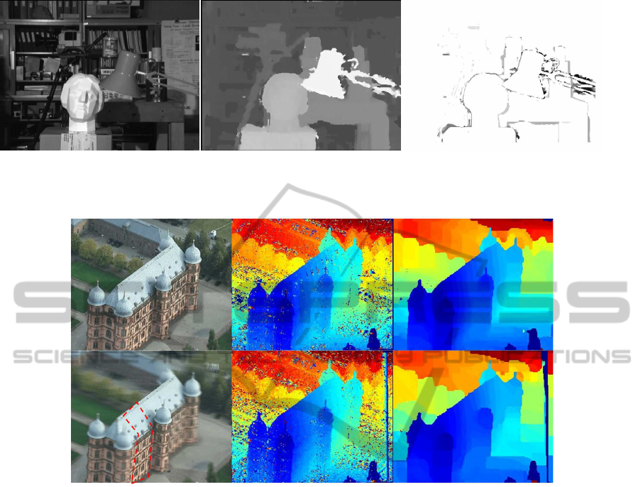
Figure 1: Performance of the plane-sweep algorithm for the data set Tsukuba with the aggregation function A3 and the
interaction set I1. On the left, the reference image. In the middle, the output depth map. On the right, absolute deviations of
disparity are shown. All pixels with deviations below one pixel are marked white.
Figure 2: Performance of the plane-sweep algorithm for the data set Gottesaue with different aggregation functions and
interaction sets. Top row: Reference image (left), result of the local method (middle), and optimization by the TRW-S method
(right) for the combination of A3+I1. Bottom row, middle and right: Analogous results for the combination A1+I2; left:
Visualization of the mean color image
ˆ
J (s) for an example value of s = 12. Pixels that approximately have this depth label lie
in the contour specified by red.
too narrow to obtain a distinctive minimum for these
structures. As follows from the visual inspection of
the results, the interaction sets I3 and I4 produce com-
parable or slightly inferior results for all aggregation
functions. For completeness, we present the reference
frame of the sequence in Fig.2, top left, and we vi-
sualize the principle of the aggregation function A5
for an example label s = 12, bottom left. We see that
in the regions where the corresponding fronto-parallel
plane intersects the surface, the image is not blurred,
in contrast to all other not homogeneously textured
regions of the reference image.
Finally, we considered several aerial videos over
the village Bonnland in Southern Germany and com-
pared the resulting depth map with a ground truth.
This ground-truth was obtained by registering the ref-
erence frame of the sequence into the coordinate sys-
tem of a very dense terrestrial laser point cloud (Bo-
densteiner and Arens, 2012). Without going into de-
tail, we report that similar observation to the Tsukuba
data set could be made. While the aggregation set A4
is a successful choice for the SAD measure, the cost
function NCC yields smaller deviations for the con-
figurations A1+I4 or A2+I4 and hence benefits from
possibly many (even redundant) observations.
5 CONCLUSIONS AND
OUTLOOK
We presented a fast and efficient multi-baseline plane-
sweep algorithm for extraction of depth maps. The al-
gorithm consists of two steps: Aggregation of radio-
metric data into a data cost matrix and non-local op-
timization. The non-local optimization module does
not represent a focus of our contribution; it presup-
VISAPP2015-InternationalConferenceonComputerVisionTheoryandApplications
400
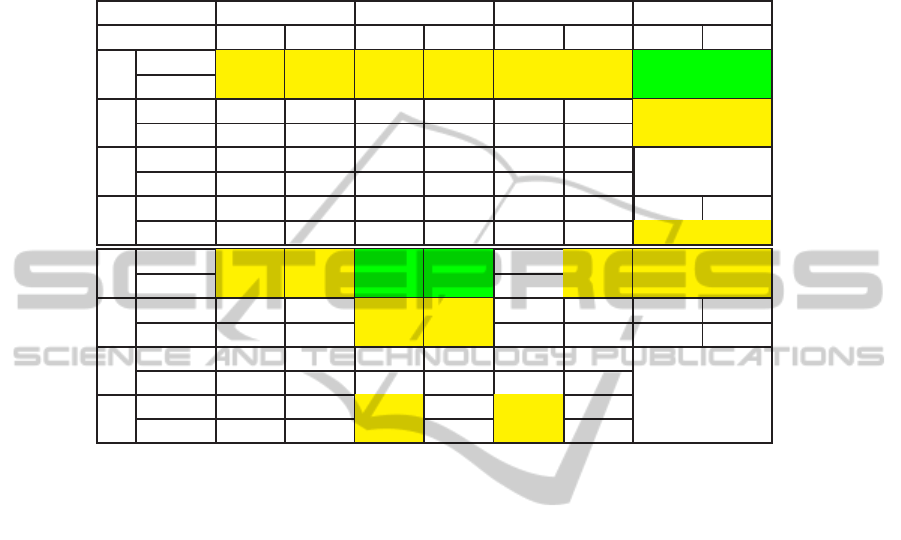
Table 1: Deviation of the calculated disparity maps to the ground truth for the data set Tsukuba with truncated SSD and
NCC data cost functions. Pixels with disparity deviations below 1 pixel are not taken into account. Five images and a
5× 5 correlation window were considered. For every meaningful pair of interaction set and aggregation function, the results
of the local algorithm and the semi-global algorithm with λ
1
= 10 and λ
2
= 20 are shown. The top number denotes the
percentages of incorrectly matched pixels while the bottom number shows these values after a neighborhood of δ = 1 (i.e.,
3× 3- neighborhood) is considered and the minimum deviation from the ground truth is extracted. The best combination of
the aggregation function and interaction set are marked in green, the relatively good ones in yellow.
A1 A2 A3 A4
param loc. SGM loc. SGM loc. SGM loc. SGM
I1
SSD, 0 4.084 3.955 4.021 3.742 4.054 3.932 3.974 3.419
SSD, 1 2.811 2.793 2.492 2.433 2.780 2.763 2.382 2.165
I2
SSD, 0 4.242 4.178 4.364 4.271 4.211 4.150 3.989 3.781
SSD, 1 3.064 3.089 2.949 2.974 3.027 3.052 2.583 2.599
I3
SSD, 0 4.564 4.543 4.734 4.616 4.523 4.494 A5
SSD, 1 3.364 3.432 3.181 3.268 3.310 3.382 no interaction
I4
SSD, 0 4.464 4.409 4.422 4.337 4.420 4.361 4.448 4.079
SSD, 1 3.213 3.237 2.892 2.947 3.166 3.189 2.761 2.737
I1
NCC, 0 4.559 4.520 4.536 4.494 5.569 4.777 4.851 4.692
NCC, 1 3.783 3.716 3.751 3.681 4.976 4.056 4.179 3.977
I2
NCC, 0 5.031 4.997 5.002 4.963 5.817 5.163 5.620 5.467
NCC, 1 4.308 4.259 4.265 4.209 5.204 4.453 5.050 4.868
I3
NCC, 0 5.151 5.123 5.124 5.087 5.400 5.216 no
NCC, 1 4.413 4.375 4.392 4.341 4.711 4.492 interaction
I4
NCC, 0 5.020 4.992 4.965 4.928 5.055 4.868
NCC, 1 4.280 4.237 4.221 4.172 4.340 4.117
poses application of one of the state-of-the-art algo-
rithms (Szeliski et al., 2006) for energy minimization
on Markov Random Fields, which are coded by the
data cost matrix and a smoothness function.
The data cost aggregation module works in arbi-
trary, not necessarily rectified configurations of im-
ages. All calculations are described as image opera-
tions: Convolutions, multiplications and divisions of
arrays, etc. The computing time of our implemen-
tation in MATLAB (this programming language is
system-accelerated while processing matrices) on a
standard PC, is around 0.5 sec.for five images, 17
depth labels and the NCC cost function (3) for the
data set Tsukuba. Moreover, it is possible to imple-
ment this module on GPU (Pollefeys et al., 2008) for
its further acceleration. The modular implementation
is easily extensible by shiftable windows, new cost
functions, mesh-based terms, etc.
Among the analyzed interaction sets and aggrega-
tion functions, we could observe from Table 1 that for
the sequence Tsukuba, differences in performance be-
tween a good and a bad choice can reach 25% if the
local result is considered, which shows the relevance
of the proposed research. The interaction sets causing
longer baselines should be chosen for more accurate
computation of depth maps. Also, a better choice of
the questioned parameters not only depends on the
geometric configuration, but also on the cost func-
tion. On the one hand, the rather distinctive SAD cost
function yields better results if there are no redundan-
cies in observations. On the other hand, if the NCC
function should be chosen because of radiometric dif-
ferences, the configurations with many observations,
e.g. A1+I4, are more promising. Implicit treating oc-
cluded pixels and border area helps to improve the
quantitative and qualitative results. Hence, the aggre-
gation function A4, tailored for smooth video streams,
works well for the data set Tsukuba. Similarly, the
aggregation function A2 turns out to be more robust
for the data set Gottesaue, captured under more turbu-
lent conditions. Besides several aggregation functions
treating pairs of images, we presented a new function
that considers all images at once. But this function is
only based on differences of gray values, and its adap-
tation for other cost functions, like NCC and Mutual
Information, should be one of our future research ar-
eas.
Finally, for evaluation of the results, we omitted
the triangle meshes in this work and only used the pre-
viously reconstructed points for initialization of mar-
gins for depth values. This is, of course, not wise
to ignore these points since consideration of triangle-
based terms and evaluation of triangles allows to re-
duce the number of mismatches. Moreover, in the
TemporalSelectionofImagesforaFastAlgorithmforDepth-mapExtractioninMulti-baselineConfigurations
401

future modifications of the algorithm, we will inves-
tigate to what extent the inclinations of triangles in
3D world could contribute to a better initialization of
planes to be swept.
REFERENCES
Belhumeur, P. (1996). A Bayesian approach to binocular
stereopsis. International Journal of Computer Vision,
19(3):237–260.
Bodensteiner, C. and Arens, M. (2012). Real-time 2D
video/3D LiDAR registration. In International Con-
ference on Pattern Recognition (ICCV), pages 2206–
2209, Tsukuba (Japan).
Boykov, Y., Veksler, O., and Zabih, R. (1998). A Vari-
able Window Approach to Early Vision. Transac-
tions on Pattern Analysis and Machine Intelligence,
20(12):1283–1294.
Bulatov, D., Wernerus, P., and Heipke, C. (2011). Multi-
view dense matching supported by triangular meshes.
ISPRS Journal of Photogrammetry and Remote Sens-
ing, 66(6):907–918.
Delong, A., Osokin, A., Isack, H. N., and Boykov, Y.
(2012). Fast approximate energy minimization with
label costs. International Journal of Computer Vision,
96(1):1–27.
Furukawa, Y. and Ponce, J. (2010). Accurate, dense, and
robust multiview stereopsis. Transactions on Pattern
Analysis and Machine Intelligence, 32(8):1362–1376.
Goesele, M., Snavely, N., Curless, B., Hoppe, H., and Seitz,
S. M. (2007). Multi-view stereo for community photo
collections. In International Conference on Computer
Vision (ICCV), pages 1–8.
Hansen, P. C. and O’Leary, D. P. (1993). The use of
the L-curve in the regularization of discrete ill-posed
problems. SIAM Journal on Scientific Computing,
14(6):1487–1503.
Heinrichs, M., Hellwich, O., and Rodehorst, V. (2007).
Efficient semi-global matching for trinocular stereo.
Photogrammetrie – Fernerkundung – Geoinforma-
tion, 6:405–414.
Hirschm¨uller, H. (2008). Stereo processing by semi-
global matching and mutual information. Transac-
tions on Pattern Analysis and Machine Intelligence,
30(2):328–341.
Hirschm¨uller, H. and Scharstein, D. (2009). Evaluation of
stereo matching costs on images with radiometric dif-
ferences. Transactions on Pattern Analysis and Ma-
chine Intelligence, 31(9):1582–1599.
Irschara, A., Rumpler, M., Meixner, P., Pock, T., and
Bischof, H. (2012). Efficient and globally optimal
multi view dense matching for aerial images. ISPRS
Annals of the Photogrammetry, Remote Sensing and
Spatial Information Sciences.
Kang, S. B., Szeliski, R., and Chai, J. (2001). Handling
occlusions in dense multi-view stereo. In Computer
Vision and Pattern Recognition (CVPR), volume 1.
Koch, R., Pollefeys, M., and Van Gool, L. (1998). Multi
viewpoint stereo from uncalibrated video sequences.
In European Conference on Computer Vision (ECCV),
pages 55–71. Springer.
Kolmogorov, V. (2003). Graph based algorithms for scene
reconstruction from two or more views. PhD thesis,
Cornell University.
Kolmogorov, V. (2006). Convergent tree-reweighted mes-
sage passing for energy minimization. Transac-
tions on Pattern Analysis and Machine Intelligence,
28(10):1568–1583.
Nakamura, Y., Matsuura, T., Satoh, K., and Ohta, Y.
(1996). Occlusion detectable stereo-occlusion pat-
terns in camera matrix. In Computer Vision and Pat-
tern Recognition (CVPR), pages 371–378.
Okutomi, M. and Kanade, T. (1993). A multiple-baseline
stereo. Transactions on Pattern Analysis and Machine
Intelligence, 15(4):353–363.
Pollefeys, M., Nist´er, D., Frahm, J.-M., Akbarzadeh, A.,
Mordohai, P., Clipp, B., Engels, C., Gallup, D., Kim,
S.-J., Merrell, P., Salmi, C., Sinha, S., Talton, B.,
Wang, L., Yang, Q., Stew´enius, H., Yang, R., Welch,
G., and Towles, H. (2008). Detailed real-time urban
3D reconstruction from video. International Journal
of Computer Vision, 78(2-3):143–167.
Rothermel, M., Bulatov, D., Haala, N., and Wenzel, K.
(2014). Fast and robust generation of semantic ur-
ban terrain models from UAV video streams. In Inter-
national Conference on Pattern Recognition (ICPR),
pages 592–597.
Scharstein, D. and Szeliski, R. (2002). A taxonomy and
evaluation of dense two-frame stereo correspondence
algorithms. International Journal of Computer Vision,
47(1):7–42.
Sun, J., Zheng, N.-N., and Shum, H.-Y. (2003).
Stereo matching using belief propagation. Transac-
tions on Pattern Analysis and Machine Intelligence,
25(7):787–800.
Szeliski, R., Zabih, R., Scharstein, D., Veksler, O., Kol-
mogorov, V., Agarwala, A., Tappen, M., and Rother,
C. (2006). A comparative study of energy minimiza-
tion methods for markov random fields. In European
Conference on Computer Vision (ECCV), pages 16–
29. Springer.
Wainwright, M. J., Jaakkola, T. S., and Willsky, A. S.
(2005). Map estimation via agreement on trees:
message-passing and linear programming. Transac-
tions on Information Theory, 51(11):3697–3717.
Zhang, H.,
ˇ
Cech, J., Wu, F., and Hu, Z. (2003). A lin-
ear trinocular rectification method for accurate stereo-
scopic matching. In British Machine Vision Conf.,
2003, pages 281–290.
VISAPP2015-InternationalConferenceonComputerVisionTheoryandApplications
402
