
MultiResolution Complexity Analysis
A Novel Method for Partitioning Datasets into Regions of Different Classification
Complexity
G. Armano and E. Tamponi
Department of Electrical and Electronic Engineering, University of Cagliari, Cagliari, Italy
Keywords:
Data Analysis, Preprocessing, Complexity, Estimation.
Abstract:
Systems for complexity estimation typically aim to quantify the overall complexity of a domain, with the
goal of comparing the hardness of different datasets or to associate a classification task to an algorithm that is
deemed best suited for it. In this work we describe MultiResolution Complexity Analysis, a novel method for
partitioning a dataset into regions of different classification complexity, with the aim of highlighting sources of
complexity or noise inside the dataset. Initial experiments have been carried out on relevant datasets, proving
the effectiveness of the proposed method.
1 INTRODUCTION
Many experimental works on classification algo-
rithms attempt to analyze the behavior of classifiers
by studying their performances on different domains.
However, the reasons behind the classifier’s success
(or failure) are rarely investigated. The connec-
tion between data characteristics and classifier design
and performance has received attention only recently
(Sohn, 1999). The aim of this emerging research area
is to discover and analyze characteristics of the data
that are related to its classification complexity.
A very simple measure of data complexity is the
accuracy (or some other performance metric) of the
adopted classifier on the dataset at hand. However,
this measure does not give any insight on the reasons
for which the classifier achieves that performance.
Moreover, theoretical studies most often reach very
loose bounds, that are not useful in practice (i.e., the
Bayes error (Fukunaga, 1990); a notable work by
Tumer (Tumer and Ghosh, 1996) aims at estimating
the Bayes error through classifiers combination).
A work by Ho details how some measures can
help discriminate an easy problem from difficult ones,
for example, average number of points per dimension,
maximum Fisher’s discriminant ratio, non-linearity of
nearest neighbor classifier (Ho and Basu, 2000). In
another work, Ho shows how to use these metrics to
select between different kinds of ensemble classifiers
for a particular classification task (Ho, 2000).
In order to find complexity measures easier to cal-
culate than the Bayes error, various authors compare
their metrics to the Bayes error itself (which is con-
sidered the golden standard). Of course, this kind of
comparison is only possible with domains for which
the Bayes error can be calculated with analytical or
numerical methods, or on datasets for which lower
and upper bounds on the Bayes error are relatively
close to one another (Bhattacharyya, 1943).
On the other hand, Singh (Singh, 2003) calcu-
lates a complexity metric by partitioning the feature
spaces into hyper cuboid, and proves the effectiveness
of his metric by showing its correlation with the per-
formance of a real classifier on unseen test data.
In the recent years, various complexity measures
have been applied to compare classifiers in order to
find the optimal classification algorithm for a given
domain (Mansilla and Ho, 2005), (Luengo and Her-
rera, 2012). In (Sotoca et al., 2006), the authors de-
scribe an automatic framework for the selection of an
optimal classifier. Finally, in (Luengo et al., 2011) the
authors apply the measures of complexity to analyze
the behavior of various techniques for imbalance re-
duction.
In general, the current literature on the topic con-
siders a dataset as a whole, to either find the most
important characterization of its complexity, as in the
case of (Ho and Basu, 2000), or to rank datasets by
their “overall” complexity.
In fact, instead of estimating the overall complex-
ity of a domain, we aim at estimating its local char-
acteristics, in order to find high-complexity regions
334
Armano G. and Tamponi E..
MultiResolution Complexity Analysis - A Novel Method for Partitioning Datasets into Regions of Different Classification Complexity.
DOI: 10.5220/0005247003340341
In Proceedings of the International Conference on Pattern Recognition Applications and Methods (ICPRAM-2015), pages 334-341
ISBN: 978-989-758-076-5
Copyright
c
2015 SCITEPRESS (Science and Technology Publications, Lda.)

inside a dataset. This can be viewed as a particu-
lar way of exploiting boundary information (Pierson
et al., 1998), which has been used in other works to
extrapolate a measure for the whole dataset (Pierson
et al., 1998).
In this work we propose MRCA (i.e., MultiReso-
lution Complexity Analysis), a method for identify-
ing regions of different complexity in a dataset. The
remainder of the paper is organized as follows: Sec-
tion 2 illustrates the proposed method for identifying
regions of different complexity. Section 3 illustrates
and discusses experimental results. Conclusions and
future work (Section 4) end the paper.
2 METHOD DESCRIPTION
Let us have a dataset defined as a set of N object-label
pairs. Each object is described by a vector of features
drawn from a feature space X . The label associated
with each object is an element of a finite set of classes
Y . We can then write D = {(x
i
, y
i
), i = 1, . . . , N}. In
the following, with a small abuse of notation, we will
write x ∈ D to refer to the feature vector of an element
in the dataset, and y(x) to refer to the observed label
associated to it. As the method we are proposed has
only been tested on binary datasets, for convenience
we will assume that Y = {−1, +1}.
A classifier for a dataset D is a computable func-
tion c which returns a predicted label for an object
given as input. In general, the form of c is indepen-
dent of the dataset, and a set of parameters need to
be set. When the predicted label differs from the true
one present in the dataset, we say that the classifier
has committed an error.
A training algorithm for a classifier c over a train-
ing dataset T (often T ⊂ D) is an algorithm which
takes the elements of T as examples to set the free
parameters of c. Often, the parameters are set to min-
imize the number of errors over the training set, but
various refinements may be used to try to reduce the
number of errors on unseen instances.
What we propose is a method to identify the inher-
ent complexity of groups of elements in the dataset, so
that it can be split into regions of different complex-
ity. We will show that the method is always capable
of separating the “hard” regions (in which the classi-
fication accuracy is always less than 50%) from the
“easy” and “average” regions.
MRCA operates according to the following steps:
1. Define a transformation able to map elements of
the given dataset to a profile space P and apply
the transformation to every element in the dataset;
2. Cluster the items in the profile space –with the un-
derlying assumption that items with similar com-
plexity occur close to each other in this space;
3. Evaluate the inherent complexity of each cluster
and rank clusters accordingto a complexity metric
called multiresolution index (MRI for short).
Our algorithm has to be applied on the “training”
part of the dataset, as it needs to know the class label
yx of each instance x.
2.1 First Step: Generating a Profile
Space
The first step is aimed at facilitating the task of esti-
mating the complexity of a sample x ∈ D. To this end,
we apply a technique called multiresolution analysis.
We estimate the complexity of the sample by drawing
around it hyper spheres of different radii. The con-
tent of each hypersphere is then analyzed by means of
a lightweight but effective complexity metric, called
imbalance estimation function. Given a set of exam-
ples D, and recalling that Y = {−1, +1} , the imbal-
ance estimation function is defined as follows:
ψ
D
(x, σ) = y(x) ·
∑
x
′
c
∈D
y(x
′
c
) · φ
σ
(x, x
′
)
∑
x
′
c
∈D
φ
σ
(x, x
′
)
∀x ∈ D
(1)
where x is the center of the current hypersphere,
whose extension is controlled by the scale factor σ,
x
′
c
is a generic feature vector in D, and φ
σ
(x, x
′
) is
a function (probe hereinafter) devised to account for
the importance of x
′
c
with respect to the object x un-
der analysis. As a design choice, the probe is also
entrusted with checking whether x
′
c
is within the cur-
rent hypersphere or not. In particular, the value re-
turned by the probe will be zero when x
′
c
is outside
it. The simplest definition for the probe would be a
sharp boundary checker, which returns 0 outside the
hypersphere and 1 inside. A more sophisticated pol-
icy would constrain φ to play the role of a fuzzy mem-
bership function, entrusted with asserting to which
extent the sample x
′
c
belongs to the probe centered in
x. In this case, a value in the range [0, 1] would be
returned when x
′
c
is inside the hypersphere, depend-
ing on its proximity with x (the closer the higher). It
can be easily shown that, by definition, ψ ranges in
[−1, +1]. In particular:
• ψ ≈ −1 indicates a strong imbalance among the
samples that occur within the probe, with labeling
mostly different from the one of x;
• ψ ≈ 0 indicates that positive and negative samples
are equally distributed within the probe;
MultiResolutionComplexityAnalysis-ANovelMethodforPartitioningDatasetsintoRegionsofDifferentClassification
Complexity
335

• ψ ≈ +1 indicates a strong imbalance among the
samples that occur within the probe, with labeling
mostly equal to the one of x.
The number of hyper spheres being m, each sam-
ple x ∈ D would be described in the profile space P
by a vector of m components. A profile p ∈ P for an
x ∈ D is obtained by repeatedly varying the scale fac-
tor in ψ, which forces the generation and evaluation
of probes with different size. The set of adopted scale
factors {σ
1
, σ
2
, . . . , σ
m
} must be drawn in accordance
with the wanted size of the profile, with the additional
constraint that σ
1
< σ
2
< . . . < σ
m
. In doing so, the
profile for a sample x ∈ D is given by:
p = [ψ
D
(x, σ
1
), . . . , ψ
D
(x, σ
m
)] = Ψ
D
(x) (2)
Applying the profile transformation Ψ to every ele-
ment in a set of instances D gives rise to a set of
profile patterns D
P
, with elements belonging to the
profile space P = [−1, +1]
m
.
We would like to stress that to apply the profile
transformation, we need both the feature vector and
the label associated with it.
2.2 Step Two: Clustering the Profile
Space
Applying centroid-based clustering to D
P
allows to
identify regions characterized by different degrees of
classification complexity. Assuming that a distance
function d is defined in P , each cluster can be iden-
tified by its proper centroid, yielding a set of r cen-
troids:
C = { p
(k)
|k = 1, 2, . . . , r } (3)
The k-th element of the underlying partition over D
P
is defined as:
D
(k)
P
= {p ∈ D
P
| f
k
(p) = 1} k = 1, . . . , r (4)
where f
k
: p → {0, 1} is the characteristic function for
the k-th cluster, which relies on the distance function
as follows:
f
k
(p) =
1 k = argmin
1≤ j≤r
d(p, p
( j)
)
0 otherwise
(5)
As for each x ∈ D a correspondent p ∈ D
P
exists, also
the original dataset D can be clustered accordingly. In
symbols:
D
(k)
= { (x, y(x))|Ψ(x) ∈ D
(k)
P
} k = 1, . . . , r (6)
2.3 Step Three: Complexity Estimation
The third step of the proposed method is aimed at es-
timating the complexity of each cluster, with the goal
of ranking them according to their complexity.
To estimate the complexity, we defined a simple
metric called Multi Resolution Index. The MRI can
be calculated for an element in D
P
or for a cluster. In
either case, it ranges in [0, 1] (the higher the value is,
the more complex the corresponding pattern or cluster
is). We decided to adopt a cumulative strategy, which
uses the first kind of MRI to evaluate the second.
As for a single pattern p ∈ P , we realized that the
components of a profile with finer granularity carry
more information about the difficulty of classifying a
pattern. To take into account this aspect, we opted
to weight the components according to the size of the
probe. In particular,the MRI of a pattern in the profile
space is defined as:
MRI(p) =
1
2m
·
m
∑
j=1
w
j
· [1− p
j
] (7)
where w
j
(j = 1, 2, . . . , m) denote weights applied
to the components of p. In particular, to imple-
ment a policy that weights more the components
with finer granularity, one may get the actual values
[w
1
, w
2
, . . . , w
m
] as samples of a monotonically de-
creasing function.
To compute the MRI of a cluster, we average the
adopted metric on the patterns that belong to the clus-
ter:
MRI
(k)
=
1
|D
(k)
P
|
·
∑
p∈D
(k)
P
MRI(p) (8)
MRI
(k)
is expected to yield small values when the k-
th cluster is characterized by a strong imbalance that
agrees with the labeling of the cluster elements them-
selves, as ψ ≈ 1. The worst case occurs when the
imbalance is against the labeling of the cluster ele-
ments, which yields MRI
(k)
≈ 1. In case of a bal-
anced cluster, MRI
(k)
≈
1
2
. As a final note on the pro-
posed method, let us point out that, by virtue of the
backward mapping between the clusters in D
P
and
the clusters in D, the ranking holds also for D
(k)
–
notwithstanding the fact that the samples correspond-
ing to the components of a cluster are typically scat-
tered along the feature space rather than being close
to each other.
3 EXPERIMENTAL RESULTS
3.1 Parameters Setting
The proposed method is customizable along several
dimensions, which are preliminarily summarized be-
low.
ICPRAM2015-InternationalConferenceonPatternRecognitionApplicationsandMethods
336

Shape of the probe. As already pointed out, we as-
sume the probe be spherically shaped
1
. According to
this assumption, a probe will be completely charac-
terized by the reference sample x and by the radius σ
of the hypersphere. The adopted probing function φ
is the boundary checker, defined as:
φ
σ
(x, x
′
) =
1 kx
′
− xk ≤ σ
0 otherwise
(9)
In agreement with Equation 9, the imbalance esti-
mation function defined in Equation 1 can be rewrit-
ten as:
ψ
D
(x, σ) = y(x) ·
N
+
σ
(x) − N
−
σ
(x)
N
+
σ
(x) + N
−
σ
(x)
(10)
where N
+
σ
(x) and N
−
σ
(x) are the number of patterns
in D with label +1 and −1 in the hypersphere with
center x and radius σ.
Distance measure. In the experiments we adopted the
Euclidean distance, defined as:
d(p, p
′
) =
s
m
∑
j=1
p
j
− p
′
j
2
p, p
′
∈ P (11)
Of course, other distance metrics are also applicable
(e.g., a la mode of p-norms).
Cardinality of the profile space. We ran the experi-
ments with multiple values for the cardinality of the
transformed space. Experiments have been run with a
value for m that falls between 10 and 50.
Scaling strategy. The radius of the probe is scaled
linearly using the scale factor σ up to the greatest
value σ
max
, which is calculated as the value of the
radius for which the corresponding hypersphere con-
tains (on average) a fixed percentage of the dataset
elements, say ρ. We ran our experiments with ρ =
0.05, 0.1, 0.15, 0.2. The expression for σ
j
is given by:
σ
j
=
j
m
· σ
max
j = 1, 2, . . . , m (12)
Weighting policy. The weighting policy has been de-
fined in accordance with the adopted scaling strategy.
We imposed a linear behavior also to this function. In
symbols:
w
j
= 1−
j − 1
m
j = 1, 2, . . . , m (13)
Partitioning strategy and cardinality of the partition.
The k-means algorithm has been adopted to imple-
ment the clustering strategy. The choice felt to k-
means, due to its simplicity among the centroid-based
1
In presence of clear differences among the dimensions
of the feature space, which can be put into evidence by cal-
culating the covariance matrix from the available samples,
one may decide to preliminarily equalize the space.
clustering algorithms. It turns out that its main limi-
tation, namely the need for specifying the number of
clusters by hand, was in fact useful in this setting. Ex-
periments have been run varying the number of clus-
ters from 3 to 5. In particular, with r = 3, we were
expecting the cluster algorithm to identify a “hard”
cluster and an “easy” cluster, together with a medium
complexity cluster.
3.2 Datasets
To assess the validity of the proposed method, we per-
formed experiments on various binary datasets. We
opted for the KEEL repository (Alcal´a-Fdez et al.,
2011), which contains several binary datasets able to
guarantee the statistical significance of experimental
results. The selected datasets are characterized as fol-
lows:
Type of features. We have selected only datasets with
only real-valued features.
Dimensionality of the feature space. With the goal of
testing the effectiveness of the proposed method on
different feature spaces, we selected datasets whose
number of features goes from 2 to 57.
The selected datasets are summarized in Table 2.
Some of them are also hosted by the UCI repository
(Bache and Lichman, 2013).
3.3 Results
We applied PCA to each dataset, reducing the num-
ber of features to 5. Then we applied a Mahalanobis
transformation on the PCA-reduced feature space, in
order to obtain a uniform covariance matrix (that is,
as a result of the two transformations the covariance
matrix of the sample becomes a 5×5 identity matrix).
On this reduced feature space, we have run our com-
plexity estimation algorithm for every combination of
the parameters shown in Table 1, for a total of 300
experiments (60 for each dataset).
In order to assess the effectiveness of the partition-
ing strategy, we checked whether a correlation exists
between the MRI of each cluster and the local com-
plexity directly estimated by means of a classifier. We
ran a 10-fold cross validation on each dataset, using
decision trees as learning algorithm (with standard
Weka (Hall et al., 2009) settings for C4.5). As perfor-
mance metrics, we evaluated accuracy, F-Score and
Matthews’ correlation coefficient for each cluster.
Figure 1 shows the relation between MRI and
accuracy when data are split into 3, 4 and 5 clus-
ters (MRI indexes have been normalized for the sake
MultiResolutionComplexityAnalysis-ANovelMethodforPartitioningDatasetsintoRegionsofDifferentClassification
Complexity
337

Table 1: Parameters used in the experiments.
Parameter Symbol Values
Profile size m 10, 20, 30, 40, 50
% of samples in maximum probe ρ 0.05, 0.10, 0.15, 0.20
Number of clusters r 3, 4, 5
Table 2: Summary of the KEEL datasets used for experi-
ments.
Name Features Size
Banana 2 5,300
Phoneme 5 5,404
Ring 20 7,400
Spambase 57 4,597
Twonorm 20 7,400
of readability). Figures 2 and 3 show the same re-
lation between MRI and, respectively, F-score and
Matthews’ correlation coefficient.
To accurately quantify the relation between MRI
and the performance metrics, we also calculated Pear-
son’s correlation coefficient for each experiment. Ta-
bles 3, 4, and 5 report the average correlation (and
confidence interval) calculated over all datasets be-
tween the MRI and accuracy, F-score and Matthews’
correlation coefficient.
Table 3: Correlation between MRI and accuracy.
m r 0.05 0.10 0.15
10
3 98.1± 1.1 98.1± 1.3 98.2± 1.3
4 97.9± 1.3 96.9± 1.9 96.3± 1.3
5 97.8± 1.5 97.0± 1.8 96.5± 1.8
20
3 98.2± 1.2 98.1± 1.3 98.3± 1.3
4 97.9± 1.3 97.2± 1.8 96.8± 1.8
5 98.0± 1.1 97.1± 2.0 96.5± 1.9
30
3 98.2± 1.1 98.1± 1.3 98.2± 1.3
4 98.0± 1.3 97.3± 1.8 96.8± 1.8
5 98.1± 1.0 97.1± 1.8 96.8± 1.9
40
3 98.3± 1.1 98.2± 1.3 98.3± 1.3
4 98.0± 1.2 97.2± 1.8 96.9± 1.8
5 98.1± 1.0 97.2± 1.7 96.7± 1.9
50
3 98.3± 1.1 98.2± 1.2 98.3± 1.3
4 98.0± 1.2 97.3± 1.8 96.9± 1.8
5 98.0± 1.0 97.2± 1.7 96.7± 1.9
3.4 Discussion
As experimental results show, MRI is always success-
ful at sorting clusters in decreasing order of classi-
fication accuracy, and its performance is stable over
Table 4: Correlation between MRI and F-Score.
m r 0.05 0.10 0.15
10
3 96.8± 2.2 96.2± 3.1 97.6± 1.3
4 97.0± 1.6 95.5± 1.7 87.0± 14.4
5 91.7± 9.0 89.0± 12.3 87.3 ± 14.9
20
3 97.0± 2.0 96.5± 2.6 97.7± 1.3
4 97.1± 1.6 95.8± 1.8 95.0± 1.9
5 92.4± 8.0 89.7± 11.8 87.6 ± 14.8
30
3 97.0± 2.0 96.5± 2.7 97.7± 1.3
4 97.2± 1.6 96.0± 1.7 95.1± 1.9
5 92.6± 8.2 90.0± 11.4 87.9 ± 14.2
40
3 97.1± 1.9 96.6± 2.5 97.7± 1.3
4 97.2± 1.6 96.0± 1.8 95.2± 1.8
5 92.6± 8.1 90.0± 11.5 88.0 ± 14.1
50
3 97.1± 1.9 96.6± 2.5 97.7± 1.3
4 97.2± 1.6 96.0± 1.7 95.2± 1.9
5 92.7± 7.7 90.0± 11.8 88.1 ± 14.1
Table 5: Correlation between MRI and Matthews’ correla-
tion coefficient.
m r 0.05 0.10 0.15
10
3 97.5± 0.6 97.1 ± 0.9 97.0± 1.2
4 96.0± 2.7 94.9 ± 2.5 93.4± 4.4
5 94.6± 5.3 92.8 ± 7.1 92.5± 6.8
20
3 97.6± 0.6 97.3 ± 0.8 97.2± 1.1
4 96.1± 2.7 95.2 ± 2.5 94.7± 2.6
5 95.1± 4.6 93.5 ± 5.9 92.6± 6.5
30
3 97.6± 0.6 97.3 ± 0.9 97.2± 1.2
4 96.2± 2.8 95.1 ± 2.8 94.7± 2.6
5 95.0± 4.9 93.3 ± 6.2 92.9± 6.6
40
3 97.6± 0.6 97.3 ± 0.8 97.3± 1.0
4 96.2± 2.7 95.2 ± 2.6 94.7± 2.6
5 95.1± 4.7 93.7 ± 5.7 93.0± 6.2
50
3 97.6± 0.6 97.3 ± 0.8 97.3± 1.1
4 96.1± 3.0 95.2 ± 2.7 94.7± 2.7
5 95.0± 4.8 92.9 ± 7.1 93.1± 6.2
a broad range of different classification domains and
configuration parameters (in particular, its perfor-
mance is clearly independent of the profile size m).
The best performance is obtained with three clus-
ICPRAM2015-InternationalConferenceonPatternRecognitionApplicationsandMethods
338
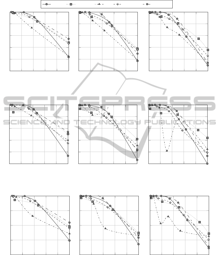
banana phoneme ring spambase
twonorm
0 1
1
MRI
Accuracy
(a) r = 3
0 1
1
MRI
(b) r = 4
0 1
1
MRI
(c) r = 5
Figure 1: MRI v. accuracy, with m = 30, ρ = 0.1.
Figure 1: MRI v. accuracy, with m = 30, ρ = 0.1.
0 1
1
MRI
F-Score
(a) r = 3
0 1
1
MRI
(b) r = 4
0 1
1
MRI
(c) r = 5
Figure 2: MRI v. F-Score, with m 30, ρ 0 1.
Figure 2: MRI v. F-Score, with m = 30, ρ = 0.1.
0 1
-1
0
1
MRI
M.C.C.
(a) r = 3
0 1
-1
0
1
MRI
(b) r = 4
0 1
-1
0
1
MRI
(c) r = 5
Figure 3: MRI v, Matthews’ correlation, with m 30, ρ 0 1.
Figure 3: MRI v, Matthews’ correlation, with m = 30, ρ = 0.1.
ters, which allow to split the dataset into hard, easy,
and medium complexity clusters. In particular, as
Figures 1a, 2a and 3a clearly highlight, the proposed
method has demonstrated very useful to identify hard
regions of the datasets in hand. In particular, the per-
formance metrics are 50% or less for “hard” clusters.
When the number of clusters increase, the corre-
lation between MRI and F-Score and Matthews’ cor-
MultiResolutionComplexityAnalysis-ANovelMethodforPartitioningDatasetsintoRegionsofDifferentClassification
Complexity
339

relation coefficient tends to be lower than the correla-
tion between MRI and accuracy. Figures 2 and 3 show
that there is actually only one outlier dataset, namely
the Ring dataset, for which we provide further discus-
sion.
The choice of ρ, the average percent of samples
embodied by the probe with greatest size, slightly in-
fluences the performance of the MRI. The reported ta-
bles show that the optimal choice is ρ = 0.05. Greater
values of ρ decrease the performance of the MRI
for ranking purposes. However, this phenomenon is
largely expected, as increasing values of ρ force the
algorithm to concentrate on greater hyper spheres,
gradually shadowing its ability of performing a local
analysis.
4 CONCLUSIONS
In this work, a method for partitioning datasets into
regions of different classification complexity has been
proposed. The method relies on a specific metric,
called MRI, which is typically used for clustering the
elements of a dataset into three regions of increasing
classification complexity, thus separating the “easy”
part of the data from the “hard” part (possibly due to
noise). Increasing the number of clusters up to five
does not decrease the ranking capacity of the MRI,
except for particular datasets and only when com-
pared with F-Score or Matthews’ correlation coeffi-
cient. Moreover, the proposed method proved to be
stable and effective for the majority of experiments
and parameter settings.
Further work on the MRI will be carried out along
both theoretical and experimental directions. Studies
on statistical significance of MRI estimates may help
to discover a lower bound on the optimal number of
clusters to be used for splitting a dataset. We are also
planning to substitute the imbalance estimation func-
tion with a local correlation estimation, aimed at sep-
arating linearly separable areas (which are typically
easy to classify), from noisy areas, as these two would
have the same imbalance but different local correla-
tion indexes.
ACKNOWLEDGEMENTS
Emanuele Tamponi gratefully acknowledges Sardinia
Regional Government for the financial support of his
PhD scholarship (P.O.R. Sardegna F.S.E. Operational
Programme of the Autonomous Region of Sardinia,
European Social Fund 2007-2013 - Axis IV Human
Resources, Objective l.3, Line of Activity l.3.1.).
REFERENCES
Abdi, H. and Williams, L. J. (2010). Principal component
analysis. Wiley Interdisciplinary Reviews: Computa-
tional Statistics, 2:433—-459.
Alcal´a-Fdez, J., Fern´andez, A., Luengo, J., Derrac, J.,
and Garc´ıa, S. (2011). Keel data-mining software
tool: Data set repository, integration of algorithms and
experimental analysis framework. Multiple-Valued
Logic and Soft Computing, 17(2-3):255–287.
Bache, K. and Lichman, M. (2013). UCI machine learning
repository.
Bhattacharyya, A. (1943). On a measure of divergence
between two statistical populations defined by their
probability distributions. Bulletin of Cal. Math. Soc.,
35(1):99–109.
Fukunaga, K. (1990). Introduction to statistical pattern
recognition (2nd ed.). Academic Press Professional,
Inc., San Diego, CA, USA.
Hall, M., Frank, E., Holmes, G., Pfahringer, B., Reute-
mann, P., and Witten, I. H. (2009). The weka data
mining software: an update. SIGKDD Explor. Newsl.,
11(1):10–18.
Ho, T. (2000). Complexity of classification problems and
comparative advantages of combined classifiers. In
Multiple Classifier Systems, volume 1857 of Lecture
Notes in Computer Science, pages 97–106. Springer
Berlin Heidelberg.
Ho, T. K. and Basu, M. (2000). Measuring the complexity
of classification problems. In in 15th International
Conference on Pattern Recognition, pages 43–47.
Luengo, J., Fern´andez, A., Garc´ıa, S., and Herrera, F.
(2011). Addressing data complexity for imbal-
anced data sets: analysis of smote-based oversam-
pling and evolutionary undersampling. Soft Comput-
ing, 15(10):1909–1936.
Luengo, J. and Herrera, F. (2012). Shared domains of com-
petence of approximate learning models using mea-
sures of separability of classes. Information Sciences,
185(1):43 – 65.
Mahalanobis, P. C. (1930). On tests and measures of group
divergence. Part 1. Theoretical formulae. Journal and
Proceedings of the Asiatic Society of Bengal (N.S.),
26:541–588.
Mansilla, E. B. and Ho, T. K. (2005). Domain of Compe-
tence of XCS Classifier System in Complexity Mea-
surement Space.
Pierson, W. E., Jr., and Pierson, W. E. (1998). Using bound-
ary methods for estimating class separability.
Pierson, W. E., Ulug, B., Ahalt, S. C., Sancho, J. L., and
Figueiras-Vidal, A. (1998). Theoretical and complex-
ity issues for feature set evaluation using boundary
methods. In Zelnio, E. G., editor, Algorithms for
Synthetic Aperture Radar Imagery V, volume 3370 of
Society of Photo-Optical Instrumentation Engineers
(SPIE) Conference Series, pages 625–636.
Singh, S. (2003). Multiresolution estimates of classifica-
tion complexity. Pattern Analysis and Machine Intel-
ligence, IEEE Transactions on, 25(12):1534–1539.
ICPRAM2015-InternationalConferenceonPatternRecognitionApplicationsandMethods
340

Sohn, S. Y. (1999). Meta analysis of classification algo-
rithms for pattern recognition. IEEE Trans. Pattern
Anal. Mach. Intell., 21(11):1137–1144.
Sotoca, J. M., Mollineda, R. A., and S´anchez, J. S. (2006).
A meta-learning framework for pattern classification
by means of data complexity measures. Inteligencia
Artificial, Revista Iberoamericana de Inteligencia Ar-
tificial, 10(29):31–38.
Tumer, K. and Ghosh, J. (1996). Estimating the bayes error
rate through classifier combining. In In Proceedings of
the International Conference on Pattern Recognition,
pages 695–699.
MultiResolutionComplexityAnalysis-ANovelMethodforPartitioningDatasetsintoRegionsofDifferentClassification
Complexity
341
