Discrete Optimal View Path Planning

Sebastian Haner and Anders Heyden

Centre for Mathematical Sciences, Lund University, Lund, Sweden

Keywords:

Path Planning, Next Best View Planning, Active Vision, Discrete Optimization, Semideﬁnite Programming,

Genetic Algorithm.

Abstract:

This paper presents a discrete model of a sensor path planning problem, with a long-term planning horizon.

The goal is to minimize the covariance of the reconstructed structures while meeting constraints on the length

of the traversed path of the sensor. The sensor is restricted to move on a graph representing a discrete set

of conﬁgurations, and additional constraints can be incorporated by altering the graph connectivity. This

combinatorial problem is formulated as an integer semi-deﬁnite program, the relaxation of which provides

both a lower bound on the objective cost and input to a proposed genetic algorithm for solving the original

problem. An evaluation on synthetic data indicates good performance.

1 INTRODUCTION

As an experimental design problem, camera network

design has been studied extensively in the photogram-

metry literature. The goal is to obtain the most accu-

rate reconstruction of a scene or object given a limited

number of observations, and the task is to ﬁnd the op-

timal set of camera poses or sensor conﬁgurations. In

robotics, the next best view problem is similarly con-

cerned with ﬁnding the next sensor position to most

improve a sequential reconstruction of the environ-

ment. Both problems are hard due to the non-convex,

multi-modal costs arising (cf. (Fraser, 1984)), but also

to the sometimes high computational burden of eval-

uating the cost function. Recent research has mostly

focused on the latter problem of accurately and efﬁ-

ciently evaluating the expected information gain of a

potential sensor conﬁguration (Low and Lastra, 2006;

Vasquez-Gomez et al., 2013; Foix et al., 2012) and

on achieving coverage of the scene (Blaer and Allen,

2007), while other works tackle minimizing the re-

sulting cost functions to ﬁnd one or a series of opti-

mal sensor conﬁgurations. As the name implies, next

best view planning usually employs a myopic plan-

ning horizon of only one step ahead, mainly due to

these difﬁculties. Camera network optimization, on

the other hand, can be seen as a long horizon plan-

ning problem, but without constraints on the order in

which observations are made.

Problems of this type have mainly been addressed

using stochastic optimization algorithms or by solv-

ing a relaxed, easier version. For example, in (Dunn

et al., 2006) the camera network problem is solved

using a genetic optimization algorithm searching the

high-dimensional parameter space of camera place-

ments. In (Wenhardt et al., 2006) the authors recon-

struct objects using a camera mounted on a robotic

arm. The object geometry is estimated using a

Kalman ﬁlter, and the next imaging location is deter-

mined by searching a discrete parameter space and

evaluating the expected information gain in the ﬁl-

ter at each position. A different approach is taken in

(Trummer et al., 2010) where the next imaging loca-

tion is decided based only on the single currently least

well-determined feature, allowing a simple closed

form solution. In (Dunn et al., 2009) the path of a

robot moving in the plane is planned based on the

expected reconstruction accuracy of an observed ob-

ject. An approximation of the geometry is given and

the expected information gain from observing the ob-

ject from a particular vantage point is determined on

a discrete grid of camera locations. Each grid cell

is assigned a cost proportional to the inverse of the

information gain, and a minimum cost path is found

between the starting point and the global minimum

grid cell. This does not take into account the fact that

an observation may be more or less valuable depend-

ing on what other observations are available, and thus

does not optimize the desired objective. In (Haner and

Heyden, 2011) a continuous optimization approach is

used to solve the similar problem of ﬁnding the best

reconstruction while also reaching a predeﬁned desti-

nation as quickly as possible, and while taking all fu-

ture observations into account, this method can only

411

Haner S. and Heyden A..

Discrete Optimal View Path Planning.

DOI: 10.5220/0005252104110419

In Proceedings of the 10th International Conference on Computer Vision Theory and Applications (VISAPP-2015), pages 411-419

ISBN: 978-989-758-091-8

 2015 SCITEPRESS (Science and Technology Publications, Lda.)

guarantee locally optimal solutions using gradient de-

scent. In this paper, we formulate discrete analogs

of the problem formulation of (Haner and Heyden,

2011) and cast them as integer semi-deﬁnite programs

(SDPs). The relaxations to continuous SDPs may be

used in a branch-and-bound scheme to ﬁnd optimal

solutions, or as input to a stochastic optimization al-

gorithm proposed below in Section 4.

Related discrete approaches include (Englot and

Hover, 2010) where a shortest path linear program

formulation similar to this work is used, but only con-

siders view coverage and not uncertainty. (Hollinger

et al., 2012) uses a two-stage approach where good

views are selected based on uncertainty, and then con-

nected by solving a traveling salesman problem.

In (Singh et al., 2009; Golovin and Krause, 2010)

approximation algorithms for the constrained path

problem using greedy strategies are shown to provide

solutions within a constant factor of the optimum,

given that the underlying cost function is submodu-

lar. Unfortunately, the maximum eigenvalue metric

used in this paper is not submodular and such guaran-

tees cannot be given; however, an optimality gap can

always be computed.

2 PROBLEM DESCRIPTION

Assume that the goal of a moving sensor is to reach

a predeﬁned target destination, while simultaneously

reconstructing its surroundings as accurately as pos-

sible, based on observations taken along the path to

the destination. There is a trade-off between reach-

ing the destination quickly, and reducing the recon-

struction uncertainty; for a bearing-only sensor such

as a camera, a longer path can accommodate more ob-

servations with greater parallax, thus improving tri-

angulation accuracy. Given a trade-off preference,

or a bound on the path length, an optimal path can

be found by solving a discrete optimization problem.

The space between and around the start and destina-

tion positions is discretized into a ﬁnite number of

possible sensor positions, and these positions consti-

tute the nodes of a graph. The edges of the graph

encode a neighborhood connectivity, i.e. the possible

motions between the ﬁxed positions. Thus a path in

the graph corresponds to a physical path. With each

node is also associated an information matrix encod-

ing how much information about the environment we

can expect to gain, if performing a measurement at

that node’s location.

The problem formulations in this paper are agnos-

tic to the graph geometry and topology, and to how

the information matrices are generated. Thus there

are no restrictions such as continuity or smoothness

on the function used to evaluate the information con-

tent of a proposed sensor conﬁguration, but which

are typically required by continuous optimization ap-

proaches. Furthermore, the information of each view

can be computed in parallel to leverage modern multi-

core processors and GPU:s.

3 PROBLEM FORMULATION

Deﬁne a directed graph G = (V,E) and a set of pos-

itive semi-deﬁnite information matrices {I

∈ S

|i =

0,... , |V|}. For a given trade-off parameter λ, deﬁne

the optimization problem

min.

p∈P

length(p) +





∑

i∈p



−1



(P1)

where P is the set of all simple paths in G from the

source node to the destination node. I

is the ini-

tially available information matrix of the environment

structure, and I

the expected information to be gained

at node i. The inverse of the information matrix is

the covariance matrix of the reconstructed structure,

so the second term measures the variance using the

scalarizing function F. This function is typically the

trace or maximum eigenvalue, corresponding to A-

and E-optimality in the experiment design literature

(Montgomery, 2000). For these choices of F, we note

that the second term is always decreasing as a func-

tion of the number of nodes on the path

. We now

make two observations: if λ is large enough, the prob-

lem is equivalent to ﬁnding the shortest path through

the graph, and may be solved efﬁciently using stan-

dard algorithms. If λ is sufﬁciently small, it is op-

timal to include all (non-zero) information matrices

in the sum, while still minimizing the distance trav-

eled, thus the problem is equivalent to the traveling

salesman problem (TSP). Since TSP is known to be

NP-hard, an efﬁcient exact algorithm for the general

case is out of reach. Also, the recognition version of

TSP (“Is there a tour of length less than L?”) is NP-

complete, so we should not expect even to be able to

verify if a given solution is optimal. This is true even

for graphs with nodes of degree at most four, e.g. pla-

nar grids (Papadimitriou and Steiglitz, 1998).

In the above formulation (P1) the parameter λ is

used to control the trade-off between a short path and

a more accurate reconstruction of the surroundings.

It is however not obvious how to select this parame-

ter, or even its suitable range, without some trial-and-

error. In fact, another problem formulation may be

This follows from the Courant-Fischer theorem.

VISAPP2015-InternationalConferenceonComputerVisionTheoryandApplications

412

more natural: given a time or distance budget, what

is the best reconstruction obtainable? In other words,

given an upper bound on the length of the path trav-

eled, minimize the reconstruction error, i.e.

min. F





∑

i∈p



−1



s.t. length(p) ≤ L .

(P2)

Note that with this formulation, as the allowed path

length grows we no longer approach TSP. Instead, for

L large enough, any Hamiltonian path on the graph

will be optimal, and for the types of graphs consid-

ered here, these are usually easily generated. Unfor-

tunately, the problem still appears difﬁcult for length

limits of practical interest. There are several other

variations on the problem formulation, for example

one could minimize the path length under the con-

straint that the covariance is reduced by a certain

amount. However, all of them appear equally hard

to solve.

Below, we derive convex relaxations of (P1) and

(P2) and show how these can be used to solve the

original problems in a branch-and-bound scheme, or

more practically as guides for more local optimiza-

tion methods. The convex relaxation and optimiza-

tion methods presented are easily adapted to alterna-

tive problem formulations.

3.1 Shortest Path as a Linear Program

The problem of ﬁnding the shortest path between two

nodes in a graph with positive edge weights is often

solved using Dijkstra’s algorithm. It can be shown

that this algorithm is equivalent to applying a primal-

dual solver to the following linear program (Papadim-

itriou and Steiglitz, 1998):

min.

∑

(i, j)∈E

s.t.

∑

j: (i, j)∈E

∑

j: (i, j)∈E

, i ∈ {1,. ..,|V| \ s,t}

∑

j: (s, j)∈E

= 1,

∑

j: ( j,t)∈E

= 1

0 ≤ x

≤ 1.

(LP)

Here x

is a variable indicating if the edge between

node i and j is part of the path or not, and c

the asso-

ciated non-negative edge weight. The constraints ex-

press ﬂow conservation, so that the number of edges

incident on a node equal the number exiting, ex-

cept for the source (s) and terminal (t) nodes which

have one outgoing and one incident edge respectively.

These constraints can be summarized into A

x = b

where A

is the |V|-by-|E| edge incidence matrix of

G with entries











−1 if edge j leaves node i

+1 if edge j enters node i

0 otherwise

, (1)

and x are the edge indicator variables suitably stacked.

It is easily shown that (LP) must have an integer opti-

mal solution. Note that this formulation does not ex-

plicitly forbid solutions consisting of a path between

the source and terminal, plus any number of closed

loops; these are only eliminated by virtue of not be-

ing optimal.

3.2 View Planning as a Semideﬁnite

Program

We adapt the shortest path problem formulation above

to the planning problem (P1). For convenience, intro-

duce binary variables α

for each node of the graph,

indicating whether that node is on the path or not. We

form the relaxed optimization problem

min.

∑

(i, j)∈E





|V|

∑

i=1



−1



s.t. A

x = b

∑

j: ( j,i)∈E

, i 6= s

= 1, 0 ≤ α

≤ 1,

(P3)

where α and x are not required to be binary. The cost

functions used in next best view planning are gen-

erally non-smooth and multi-modal, and difﬁcult to

optimize. However, due to the discretization, the ar-

gument to the second term of the objective above is

afﬁne in α. Both the trace-of-inverse and maximum

eigenvalue-of-inversefunctions are convex,and using

the epigraph trick the second term may be formulated

as a convex semideﬁnite constraint (see e.g. (Boyd

and Vandenberghe, 2004)). As one would expect, this

semideﬁnite program no longer has all the desirable

properties of the linear program; integrality of x or α

is no longer guaranteed, and a solution with disjoint

loops may in fact be optimal.

The corresponding convex relaxation of (P2) is

the same as (P3), except that the ﬁrst term of the

objective is transformed into a linear inequality:

min. F





|V|

∑

i=1



−1



s.t. A

x = b

∑

(i, j)∈ E

≤ L

∑

j: ( j,i)∈E

, i 6= s

= 1, 0 ≤ α

≤ 1.

(P4)

DiscreteOptimalViewPathPlanning

413

Selecting L is more intuitive than choosing λ; one

must only be careful not to produce an infeasible

problem by selecting L too low, but the lower limit

is readily obtained using a standard shortest path al-

gorithm.

It is possible to ﬁnd an optimal integer solution

to (P3) or (P4) using a standard branch-and-bound

search, but this is also known to be NP-hard and

may take a large number of iterations, each involv-

ing solving a potentially quite large SDP. If a solu-

tion is found, it may also contain unwanted disjoint

loops. While it is easy to include linear constraints

forbidding any particular loop in the SDP, since there

are exponentially many possible loops in the graph,

adding constraints against them all at the outset is in-

feasible. But, they can be added on an as-needed ba-

sis; if loops are present in the solution, add constraints

against them and solve again until no loops remain.

As it turns out, 2-cycles are quite common in the so-

lutions, and as their number is typically linear in the

number of nodes, it is feasible to remove them at the

outset which may lead to faster convergence to a loop-

free solution.

Obviously, the above procedure may be very time

consuming or completely intractable for all but the

smallest problem instances. However, we also noted

above that depending on the trade-off parameter λ,

the original problem (P1) should vary in difﬁculty

between simple shortest path (typically O (|E|log|V|)

for Dijkstra’s) up to exponential complexity. Em-

pirically, it turns out that many instances are in fact

“easy”, in that very few steps of branch-and-bound

are required and few or no loops are included in the

solution. Yet, many other instances are indeed difﬁ-

cult and not amenable to this approach.

4 APPROXIMATE SOLUTION

Despite the problems of tractability in ﬁnding optimal

solutions described above, it can be noted that the re-

laxed SDP formulations (P3) and (P4) provide lower

bounds on the optimal objective values of (P1) and

(P2). This may be used to verify the performance of

approximation algorithms. Also, if the problem in-

stance at hand is “easy enough”, the relaxed solution

∗

may be quite close to a valid integer, loop-free so-

lution. In these cases it is possible to construct a valid

solution to (P1) using a simple shortest path search

on the graph G with edge weights c

= 1− x

∗

. This

solution may be good enough, or can serve as initial-

ization for local or stochastic optimization algorithms.

For the formulation (P2) a slightly different approach

is needed, which will not be explored here.

4.1 A Simpliﬁed Formulation

Given the hardness of (P1) and (P2), it is natural to

seek a simpliﬁed problem formulation which might

admit faster solution algorithms. Part of the difﬁculty

is the nonlinearity of the interaction between the in-

formation matrices when taking the inverse to obtain

the covariance; the value of any particular contribu-

tion to the information depends on all the others. For-

going this interaction, instead of minimizing the co-

variance, one can maximize the trace of the informa-

tion matrix, yielding the problem

min.

p∈P

length(p) −

trace



∑

i∈p



(P5)

Since the trace is linear, this results in a shortest

path problem on G with modiﬁed weights (subtract

trace(I

)/λ from each edge incident on node i). As

long as this does not result in any negative cycles,

this may be efﬁciently solved using e.g. the Bellman-

Ford algorithm, or even Dijkstra’s if all weights are

non-negative. If negative cycles are present, the prob-

lem again becomes much more difﬁcult. In the ex-

treme where all edge weights are negative, the prob-

lem is equivalent to the longest simple path problem

on −G, which is known to be NP-hard (Schrijver,

2004). Unfortunately, for many scenarios and reason-

able choices of λ negative cycles will be present, and

in these cases (P5) can be formulated as (LP) but with

binary constraints on x. While this ILP may be signif-

icantly faster to solve than (P3), the complexity is the

same and no-loop constraints must also be introduced

incrementally. However, in some scenarios it may be

reasonable to restrict the graph G to be acyclic, and

then the shortest path problem can always be solved

in linear time. A general graph may be reduced to a

directed acyclic graph by ordering the nodes by de-

creasing distance to the target node, and only keeping

edges reducing the distance, thus forcing the sensor

to move monotonically towards the destination. This

will of course not work for purely exploratory scenar-

ios where the start and end points may be near.

Even with this signiﬁcantly simpliﬁed formulation

sacriﬁcing the interdependence of measurements, the

problem is still not easy in general. We therefore in-

troduce a stochastic genetic algorithm applicable to

all problem formulations.

4.2 A Genetic Algorithm

Genetic algorithms (GA) are a class of evolutionary

optimization algorithms which emulate the process of

natural selection. A population of candidate solutions

is maintained, and in every iteration of the algorithm,

VISAPP2015-InternationalConferenceonComputerVisionTheoryandApplications

414

a new population is generated by mutation and cross-

ings of individuals of the previous generation. The

chance of an individual producing offspring in the

next generation is proportional to that individual’s ﬁt-

ness, calculated from the corresponding value of the

function being minimized. Genetic algorithms have

been found to be quite efﬁcient in providing good so-

lutions to many combinatorial optimization problems,

including TSP (Choi et al., 2003; Schmitt and Amini,

1998) and path planning (Davoodi et al., 2013), which

motivates the use here.

To use a genetic algorithm, one must choose a rep-

resentation for a candidate solution, and deﬁne unary

mutation and binary crossover operators. In this work,

each individual is described simply as a sequence of

vertices constituting the path. The GA framework

used is completely standard; for brevity we describe

only the important steps below.

Initialization The ﬁrst step is to generate candidate

solutions, in this case paths in G from the source to

the terminal node. Unless we have some a priori in-

formation on the characteristics of the optimal solu-

tion, these should be spread out uniformly across the

space of all feasible paths. Unfortunately, truly uni-

form sampling of simple paths on a general graph ap-

pears to be a difﬁcult problem. Reasonably random

paths, however, may be obtained using random order

depth-ﬁrst search (DFS), loop-erased random walk

(Lawler, 2012), or for undirected graphs by comput-

ing the minimum cost spanning tree with randomized

edge weights, and extracting the unique path in the

tree. If candidate solutions have been obtained using

any of the heuristic methods based on the SDP relax-

ation, these can be included in the initial population

and will then be reﬁned.

Mutation Operators A mutation operator should

introduce “noise” or randomnessinto an existing path,

while preserving its main features. In practice, sev-

eral mutation operators are often employed, exploit-

ing problem-speciﬁcheuristics. To modify a path, just

randomly replacing vertices is not possible, since not

every sequence of vertices is a valid path in the graph

G. Instead, our ﬁrst operator selects two random cut

points along the path, and replaces the path in be-

tween with a random one generated using either ran-

domized DFS or loop-erased random walk. A second

operator instead replaces the section with the short-

est path between the cut points. This is motivated by

the fact that optimal paths are often quite regular, so

it makes sense to smooth out kinks. Both these oper-

ators are comparatively slow, so we also use a much

faster but more local operator which simply selects a

random vertex on the path, and replaces it with one

picked from the intersection of nodes reachable from

the preceding node with those with outgoing edges

incident on the next node on the path.

Crossover Operator The crossover operator takes

two existing paths as input and producesa mixed path,

containing parts of both, assuming they cross at some

point. This is accomplished by selecting a random

simple path on the graph obtained from G consisting

only of the edges on the two paths.

Local reﬁnement To speed up convergence to a lo-

cally optimal solution, paths may be optimized by

systematically applying the fast local mutation oper-

ator described above in a deterministic fashion. Each

node on the path, visited in random order, is re-

placed with the neighbor which minimizes the objec-

tive function.

With the formulation (P2), we run the risk of gen-

erating infeasible paths in the course of the genetic

algorithm. A simple solution is to reject any infeasi-

ble path obtained and repeat the mutation or crossover

operation until a feasible realization is produced. It is

easy to verify that if the inputs are feasible, the oper-

ators deﬁned above will eventually produce feasible

output. However, depending on how close L is to the

lower bound of feasibility, this may take an unreason-

able amount of time. The very simplest solution is to

transform the length constraint to a hard penalty term

in the objective, e.g.

min. F





∑

i∈p



−1



+ B

{p : length(p)≤L}

(2)

where B

is the barrier function for the set S s.t.

B(x) = 0 if x ∈ S and ∞ otherwise.

5 STRATIFIED SOLUTION

STRATEGY

The genetic algorithm will quickly ﬁnd good solu-

tions if the search space is not too large. For large

grids with many hundreds of nodes and large neigh-

borhood connectivities, the algorithm risks getting

stuck in local optima, often producing implausible-

looking paths. We therefore propose to reduce the

search space by substituting a smaller graph, based on

the solution of the SDP relaxation of the problem, to

obtain a good initialization which can then be reﬁned

on the full graph.

DiscreteOptimalViewPathPlanning

415

5.1 Reducing the Graph

The idea is to keep only a subset of the N most impor-

tant nodes, as indicated by the fractional SDP solu-

tion α

∗

. Interpreting these values as probabilities, we

draw N nodes without replacement, selecting nodes in

proportion to their α

∗

-value. The reduction in the co-

variance achieved using only these nodes is computed

and maximized through repeated random sampling of

the subset.

Once a subset has been chosen, a new fully con-

nected graph is formed, where edges between the

nodes represent the shortest path between them in the

original graph. This allows the mapping of paths on

the reduced graph to the full graph where they can

be evaluated. The genetic algorithm can now be run

without modiﬁcation on the reduced graph, where the

parameter N can be chosen to trade ﬁdelity for con-

vergence speed.

6 EXPERIMENTS

Due to the general formulation of the basic problem,

many different scenarios can be accommodated by

adapting the graph G and edge weights c

, which

do not need to fulﬁll geometric constraints such as

the triangle inequality. For example, each node can

represent a camera position and an orientation, and

the connectivity between poses can be deﬁned so as

to constrain angular velocity on the path. Purely ex-

ploratory behavior can be achieved by selecting start

and/or destination nodes as “super-nodes” connected

to every other node with zero weight, thus effectively

permitting arbitrary start and destination points. Typi-

cally, we know less about the scene further away from

the starting point, so the predictions of what will be

seen, or what obstacles lay ahead, may be incorrect.

Therefore one should plan with caution; by weight-

ing the information matrices based on distance to the

starting node, such behavior can be incorporated.

In the synthetic experiments below, each node

(except super-nodes) has an associated camera pose

deﬁning position and orientation. The environment

structure is represented by 3D points, each consid-

ered independently estimated such that the initial

information matrix I

is block diagonal (in fact we

let it be the identity matrix so that the uncertainty

is on the order of the scene scale). To compute the

information gained from acquiring an image at a

certain pose, the standard pinhole camera model is

used, so that the relation ˆx = f(P,X) between a world

point X and its projection ˆx is given by

Figure 1: Cameras looking at a point cloud are placed on an

8-connected unit grid. Top left, the greenness and thickness

of edges is proportional to x

∗

, the corresponding variable

of the solution to the relaxed SDP (P3), using the maxi-

mum eigenvalue scalarizing function and λ = 2. Due to the

symmetry of the problem, both a left and right path seem

to be given equal consideration. The lower bound obtained

is 61.1. Top right, the same problem with the path (green)

found by the genetic algorithm among possible positions

(blue), with a cost of 67.3. The third plot shows the same

problem but with λ = 40 and ﬁnal cost 32.6, as compared

to the lower bound of 23.0. Depending on problem charac-

teristics, bounds may be more or less tight.

f(P,X) =



X + P



⊤

(3)

where P

is the i:th row of the camera matrix. Given

a point

X, the corresponding block of I

is computed

as J

⊤

−1

J, where J =

d f



is the projection Ja-

cobian and Σ the assumed measurement error covari-

ance on the image plane. However, if

X is out of the

camera’s ﬁeld of view or too far away, the block is set

to zero. In Fig. 1–5 different experiments are shown

;

the details of the setup and results are in the ﬁgure

captions. Note that in these experiments, the online

nature of the problem is not demonstrated; in real use,

as the sensor moves and new information becomes

available, the structure and uncertainties need to be

updated and the path re-planned. By seeding the op-

timizer at each stage with the previous solution, rapid

convergence is possible.

6.1 Practical Considerations

The choice of scalarizing function F can have a large

impact on the solution time of the SDP, depending on

Many of the plots in the PDF version of this paper are embed-

ded 3D models which may be viewed on-screen in recent versions

of Adobe Reader.

VISAPP2015-InternationalConferenceonComputerVisionTheoryandApplications

416

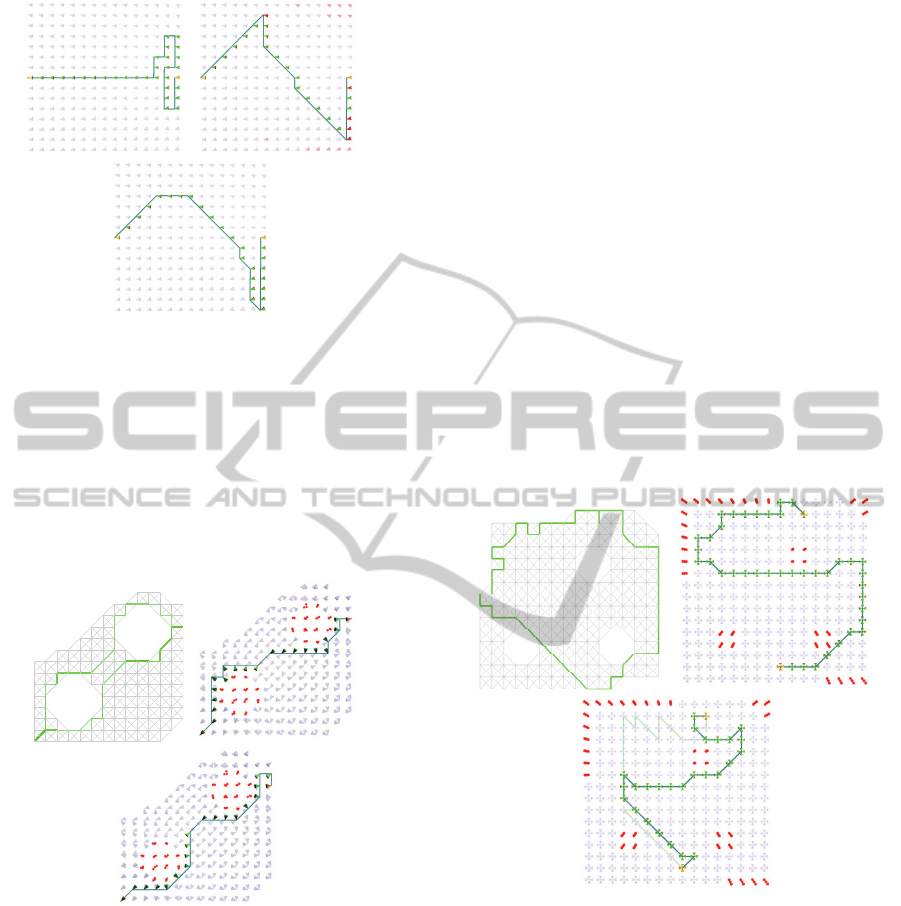
Figure 2: The same situation as in Fig. 1, now solving prob-

lem (P2) with L = 30. Top left, the solution obtained by

solving the analog of the simpler problem (P5), giving a

cost of 92.3 compared to the SDP lower bound of 67.7. Top

right, the red nodes indicate the reduced graph obtained by

sampling the SDP solution with N = 20, and applying the

GA gives a path with cost 88.7. In the bottom plot, the GA

run on the full graph with cost 86.36. The simpliﬁed formu-

lation is qualitatively different from the others and focuses

on getting as close to the structure as possible while ne-

glecting the parallax effects. It is therefore not a suitable

approximation in many situations.

Figure 3: In this example, two nodes each are placed in

every point of an 8-connected unit grid. The two nodes rep-

resent a camera looking at either of two objects/obstacles.

Top left, the solution to the relaxed SDP (P4), using the

trace scalarizing function and L = 22. Nodes of the original

square grid whose combined shortest distance to the start

and destination nodes is greater than L have been removed,

since they cannot be part of a feasible solution. As in Fig. 1,

there appears to be two competing paths, with edge values

∗

≈ 1/2. Top right, the path obtained from the simpliﬁed

formulation (P5), which works reasonably for this problem

instance. In the bottom plot, the solution obtained using the

proposed genetic algorithm. The corresponding objective

values are 192.1, 271.8 and 262.1. The gap between the

ﬁnal objective and the lower bound given by the SDP is rel-

atively large, but the path obtained directly from the SDP

solution is still quite reasonable.

the dimension of the information matrices. To mini-

mize the trace of the covariance matrix, one variable

per eigenvalue is required, while the maximum eigen-

value cost only needs one. On the other hand, eval-

uating the trace cost function is typically faster. Fur-

thermore, the maximum eigenvalue is vulnerable to

outliers e.g. features which are not seen in any or too

few views. If such features are not removed in a pre-

processing step, the cost function can never decrease

below the initial uncertainty.

The algorithms were implemented in Matlab with

core functions in MEX C++. SDPs were set up us-

ing YALMIP (L¨ofberg, 2004) and solved using the

MOSEK interior-point optimizer (Dahl, 2012). For

the experiment in Fig. 4, solving the SDP with the

trace cost took 8.7 s as opposed to 4.2 s for the max-

imum eigenvalue, while the genetic algorithm (on the

full problem) runs at about 10 iterations per second on

the same Core 2 Duo 3.0 GHz computer, with a pop-

ulation of 60 individuals. With parallel processing of

individuals, speed can likely be increased manyfold.

Figure 4: In this experiment, we simulate an omnidirec-

tional camera by adding the information matrices of four

cameras at each location. Each cluster thus corresponds to

only one node of the graph. Top left, the SDP (P4) with

L = 43 gives a lower bound at 4.11. Top right, the solution

using the stratiﬁed approach, with cost 5.47. In the last plot,

the graph has been reduced to a DAG such that the observer

must move towards the target at every step. This limits the

search space making branch-and-bound tractable, the opti-

mal solution with cost 17.98 is shown next to the solution

of the simpliﬁed problem (P5) (pale green) with cost 30.81.

DiscreteOptimalViewPathPlanning

417

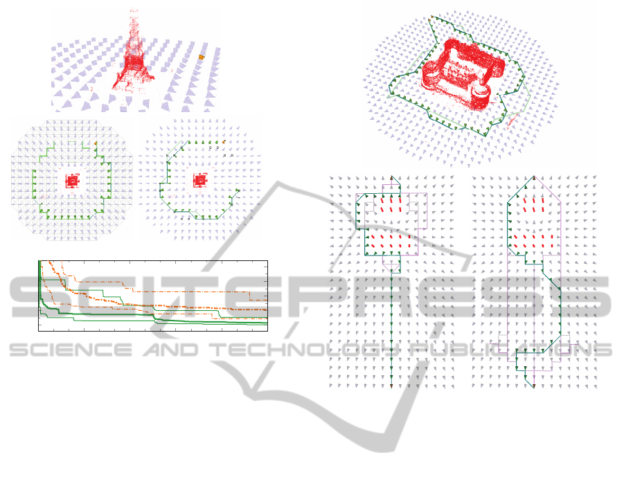
0 100 200 300 400

500

2.5

3.5

4.5

Iteration number

Φ(p)

Figure 5: Exploratory scenario with ﬁxed start and free end

point. The point cloud of the monument has been reduced

to a few hundred representative points (by random sam-

pling) to constrain the information matrix dimension. In

the middle left plot, the SDP solution giving lower bound

1.76 along with the “ﬁlled in” path found as the shortest

path on the graph with weights 1− x

∗

(see Section 4), hav-

ing cost 3.18. Middle right, the GA solution on the reduced

graph obtained by sampling the SDP solution, with nodes

marked with black squares, shown in light green with cost

2.78. The dark green path is the result of the GA on the

full graph, seeded with the reduced solution, with cost 2.57.

Achieving similar cost using random initialization takes sig-

niﬁcantly longer; the bottom graph shows the progression of

the objective value (Φ) over iterations of the proposed ge-

netic algorithms. The orange dashed curves show the max-

imum, minimum and median over 20 runs of the GA on

the full graph with random initialization. The green curves

show the same for the stratiﬁed approach, ﬁrst running 250

iterations on the reduced graph, then switching to reﬁne-

ment on the full graph. It is clear that the stratiﬁed scheme

converges much faster.

7 CONCLUSIONS

While the general problems considered in this paper

are demonstrably hard, satisfactory solutions can be

found sometimes directly from the SDP relaxation,

and often by the proposed genetic algorithm. In many

scenarios, the SDP solution gives hints as to what a

good path might look like, while in others it consists

of seemingly random, disconnected edges only. In

those cases the lower bound obtained is usually not

Figure 6: Top: stratiﬁed algorithm run on castle dataset, re-

duced to one hundred representative points using random

sampling. Bottom right: same scenario as on the left, but

here the information matrix at each node has been down-

weighted by the distance from the start node, to signify re-

duced conﬁdence in future measurements. The pale purple

lines indicate the SDP solution, the green path the GA solu-

tion.

very tight and it is difﬁcult to draw any conclusions

about the optimality of any path. This is of course to

be expected given the hardness of the problem. Nev-

ertheless, the SDP solution can always be used to seed

the GA optimizer in the proposed three-stage strati-

ﬁed algorithm.

The linearized approximation (P5) sometimes

gives reasonable solutions, as in Fig. 3, but most

often does not show any proper long-term planning

behavior, as in Fig. 2. On a directed acyclic graph

(Fig. 4 right) it does have the advantage of being

extremely fast compared to the other methods.

For computational tractability, structure points

must be considered independent, and real point cloud

data need to be subsampled. How to best subsample

while preserving data characteristics has not yet

been considered. As the graph size and connectivity

increases, computational complexity also rises and

the quality of solutions attainable in reasonable time

drops. This limits the resolution of the discretization,

particularly in the orientation space, which means

VISAPP2015-InternationalConferenceonComputerVisionTheoryandApplications

418

local, continuous reﬁnement may be a desirable

second step. This we leave to future work.

Full source code to replicate the exper-

iments in this paper are available at http://

github.com/sebhaner/nbv

discrete.

REFERENCES

Blaer, P. and Allen, P. (2007). Data acquisition and view

planning for 3-d modeling tasks. In Intelligent Robots

and Systems, 2007. IROS 2007. IEEE/RSJ Interna-

tional Conference on, pages 417–422.

Boyd, S. and Vandenberghe, L. (2004). Convex Optimiza-

tion. Cambridge University Press, New York, NY,

USA.

Choi, I.-C., Kim, S.-I., and Kim, H.-S. (2003). A genetic

algorithm with a mixed region search for the asym-

metric traveling salesman problem. Computers & Op-

erations Research, 30(5):773 – 786.

Dahl, J. (2012). Semideﬁnite optimization using MOSEK.

In 21st International Symposium on Mathematical

Programming.

Davoodi, M., Panahi, F., Mohades, A., and Hashemi, S. N.

(2013). Multi-objective path planning in discrete

space. Applied Soft Computing, 13(1):709 – 720.

Dunn, E., Olague, G., and Lutton, E. (2006). Parisian cam-

era placement for vision metrology. Pattern Recogni-

tion Letters, 27(11):1209–1219.

Dunn, E., van den Berg, J., and Frahm, J.-M. (2009). Devel-

oping visual sensing strategies through next best view

planning. In Intelligent Robots and Systems, 2009.

IROS 2009. IEEE/RSJ International Conference on,

pages 4001–4008.

Englot, B. and Hover, F. (2010). Inspection planning for

sensor coverage of 3d marine structures. In IROS,

pages 4412–4417. IEEE.

Foix, S., Kriegel, S., Fuchs, S., Aleny, G., and Torras, C.

(2012). Information-gain view planning for free-form

object reconstruction with a 3d tof camera. In Ad-

vanced Concepts for Intelligent Vision Systems, vol-

ume 7517 of Lecture Notes in Computer Science,

pages 36–47. Springer Berlin Heidelberg.

Fraser, C. S. (1984). Network Design Considerations for

Non-Topographic Photogrammetry. Photo Eng. and

Remote Sensing, 50(8):1115–1126.

Golovin, D. and Krause, A. (2010). Adaptive submodular-

ity: A new approach to active learning and stochastic

optimization. In 23rd Annual Conference on Learning

Theory, pages 333–345.

Haner, S. and Heyden, A. (2011). Optimal view path plan-

ning for visual SLAM. In Heyden, A. and Kahl, F., ed-

itors, Image Analysis, volume 6688 of Lecture Notes

in Computer Science, pages 370–380. Springer Berlin

/ Heidelberg.

Hollinger, G. A., Englot, B., Hover, F., Mitra, U., and

Sukhatme, G. S. (2012). Uncertainty-driven view

planning for underwater inspection. In ICRA, pages

4884–4891. IEEE.

Lawler, G. (2012). Intersections of Random Walks. Modern

Birkh¨auser Classics. Springer-Verlag New York.

L¨ofberg, J. (2004). Yalmip : A toolbox for modeling and

optimization in MATLAB. In Proceedings of the

CACSD Conference, Taipei, Taiwan.

Low, K.-L. and Lastra, A. (2006). An adaptive hierarchi-

cal next-best-view algorithm for 3d reconstruction of

indoor scenes. 14th Paciﬁc Conference on Computer

Graphics and Applications, Taipei, Taiwan.

Montgomery, D. C. (2000). Design and Analysis of Exper-

iments. John Wiley & Sons Canada, Ltd., 5th edition.

Papadimitriou, C. H. and Steiglitz, K. (1998). Combinato-

rial Optimization: Algorithms and Complexity. Dover

Publications.

Schmitt, L. J. and Amini, M. M. (1998). Performance

characteristics of alternative genetic algorithmic ap-

proaches to the traveling salesman problem using path

representation: An empirical study. European Journal

of Operational Research, 108(3):551 – 570.

Schrijver, A. (2004). Combinatorial Optimization : Polyhe-

dra and Efﬁciency (Algorithms and Combinatorics).

Springer.

Singh, A., Krause, A., Guestrin, C., and Kaiser, W. J.

(2009). Efﬁcient informative sensing using multiple

robots. J. Artif. Intell. Res. (JAIR), 34:707–755.

Trummer, M., Munkelt, C., and Denzler, J. (2010). Online

Next-Best-View Planning for Accuracy Optimization

Using an Extended E-Criterion. In Proc. International

Conference on Pattern Recognition (ICPR’10), vol-

ume 0, pages 1642–1645. IEEE Computer Society.

Vasquez-Gomez, J. I., Sucar, L. E., and Murrieta-Cid, R.

(2013). Hierarchical ray tracing for fast volumetric

next-best-view planning. 2013 International Confer-

ence on Computer and Robot Vision, 0:181–187.

Wenhardt, S., Deutsch, B., Hornegger, J., Niemann, H., and

Denzler, J. (2006). An Information Theoretic Ap-

proach for Next Best View Planning in 3-D Recon-

struction. In Proc. International Conference on Pat-

tern Recognition (ICPR’06), volume 1, pages 103–

106. IEEE Computer Society.

DiscreteOptimalViewPathPlanning

419