
Context-sensitive Filtering of Terrain Data based on Multi Scale Analysis
Steffen Goebbels and Regina Pohle-Fr¨ohlich
Faculty of Electrical Engineering and Computer Science, Niederrhein University of Applied Sciences,
Reinarzstr. 49, 47805 Krefeld, Germany
Keywords:
Surface Triangulation, Polygon Count Reduction, Wavelet Transform.
Abstract:
This paper addresses triangle count reduction for regular terrain triangulations. Supported by additional infor-
mation available from cadastre data, non-linear low pass filtering based on wavelet coefficients is applied. The
aim is to generate a simplified view of a city model’s terrain so that still landmarks can be easily recognized.
Height data, that are not critical for visual impressions, are compressed with lower resolution than height data
belonging to landmarks. Results are presented for the German city of Krefeld.
1 INTRODUCTION
Airborne laser scanning of terrain results in a huge
amount of vertices that is not immediately suitable
for drawing a surface triangulation. In this paper an
approach is discussed where additional information
from register data about ground usage is used for data
reduction. From that information we derive precision
that is necessary to draw certain areas. Goal is that the
terrain still should be recognizable while the number
of triangles is minimized.
Wavelet transforms are an often used method for
point cloud compression, filtering and extraction of
bare earth, cf. (Vu and Tokunaga, 2004; Wei and Bar-
tels, 2006; Xu et al., 2007; Hu et al., 2014). Besides
polygon merging, polygon elimination, vertex elim-
ination, edge collapsing, and different retiling tech-
niques, multi-resolution wavelet analysis is one of
the main methods for mesh reduction, cf. (Kalber-
matten, 2010, pp. 45–77), (Mocanu et al., 2011;
W¨unsche, 1998; Wiman and Yuchu, 2009). For ex-
ample (Olanda et al., 2014; Bjørke and Nilsen, 2003;
Bruun and Nilsen, 2003) give an overview of wavelet
techniques for simplification of digital terrain mo-
dels. These techniques do not use additional infor-
mation besides height data. Studies were carried
out with biorthogonal average interpolating wavelets.
The property of conserving average height values at
different scales yields good approximationsof terrain.
As wavelet transform allows for local frequency
filtering, it is predestined for local, context-sensitive
data reduction. However, knowledge of local proper-
ties of ground is needed. For example, good visible
sharp edges can be detected from height data using
curvature coefficients. Such edges should be main-
tained and not eliminated by filtering. In the example
of a city model we do not have to detect such patterns
in height data as we can use additional information
from a geographic information system (GIS)
1
. These
cadastre data describe ground usage in terms of poly-
gons that stand for streets, railway lines, bridges, etc.
This approach to local filtering based on digital maps
has been proposed before, for example in (Mahler,
2001, p. 58) in the context of coast lines. New is a set
of heuristic rules to determine the local level of filter-
ing using a simple filtering algorithm that differenti-
ates between low frequencies describing terrain on a
coarse scale and high frequencies needed for details.
Whereas for example in (Bjørke and Nilsen, 2003)
one biorthogonal wavelet transform is used to filter
the whole frequencyspectrum, we apply two different
transforms to minimize triangle count:
Local areas like embankments, shallow hills and
heaps that afford a higher quality of rendering will
be filtered using the simplest average interpolating
wavelet that is the discontinuous Haar wavelet. We
apply non-linear filtering using thresholds for wavelet
coefficients. In our scenario the work with continuous
orthogonal or biorthogonal wavelets is not necessary.
In contrast, local support of the Haar wavelet helps to
be very location specific.
Haar wavelet transform leads to artifacts like visi-
ble steps if only low frequencies remain after filtering.
Therefore, areas which do not require detailed ren-
1
Case study is based on geographical data, which are
protected by copyright: Geobasisdaten der Kommunen und
des Landes NRW
c
Geobasis NRW 2014.
106
Goebbels S. and Pohle-Fröhlich R..
Context-sensitive Filtering of Terrain Data based on Multi Scale Analysis.
DOI: 10.5220/0005252201060113
In Proceedings of the 10th International Conference on Computer Graphics Theory and Applications (GRAPP-2015), pages 106-113
ISBN: 978-989-758-087-1
Copyright
c
2015 SCITEPRESS (Science and Technology Publications, Lda.)

dering will be low pass filtered via continuous linear
spline approximation (that also can be interpreted as
a biorthogonalwavelet transform based on B-splines).
To be more specific, we do this spline based low pass
filtering for the whole scenario and not only for ar-
eas with little detailed information. Reason is, that
local areas with relevant details are not only detected
heuristically on the basis of context information but
also based on deviations between the surface of spline
approximation and unfiltered heights. For these ar-
eas we triangulate with heights obtained from filtering
with the Haar wavelet. Otherwise, heights for trian-
gulation are taken from spline approximation. Spline
approximation gives us a degree of freedom to fur-
ther decrease triangle count while preserving a more
detailed triangulation of areas that are displayed in
higher quality. We modify the precision of spline in-
terpolation to find a minimum number of triangles.
2 TRIANGULATION BASED ON
FILTERED HEIGHTS
Our algorithm consists of two steps. In the first step,
height data are filtered with spline approximation and
wavelet transform as described in subsequent sec-
tions. In a second step, mesh simplification can be
performed more efficient due to the adjusted heights.
For the second step a variety of well established algo-
rithms like edge collapsing can be used, cf. (Garland
and Heckbert, 1997; Silva and Gomes, 2004). Also,
the simplification can be made dependent on distance
to the viewer by using geometry clipmaps as intro-
duced in (Losasso and Hoppe, 2004). However, to test
our approach we decided to use a very basic algorithm
that is described in this section. The algorithm works
with an equidistant mesh where 400 square kilometers
are represented by (5 ·2
9
+ 1)
2
grid points. Triangu-
lation is done for each square kilometer separately on
the basis of squares that are split up into two triangles
using a diagonal. We divide a square recursively into
four smaller squares of equal size in case the surfaces
of triangles deviate more than ε from previously fil-
tered heights. A predefined accuracy level ε = 0.2 m
is a good compromise fitting with the accuracy of un-
derlying laser scanning data, but we also show num-
bers for ε = 0.05 and ε = 0.1 m. Because mesh con-
nectivity changes, larger ε might lead to visible gaps
between surface triangles.
To avoid unsightly edges when displaying diag-
onal structures, we use following rule to choose the
diagonal for splitting up a square into two triangles.
We compute the four absolute differences between the
arithmetic mean of all four heights of square vertices
Figure 1: Triangulation based on an equidistant mesh.
and each of the four heights. If P is a vertex with a
maximum difference, then we select the diagonal for
which P is not end point. Further down, this rule is
described with formula (1). Because no orientation of
the diagonal is a-priori favored over the other, we do
not get a type-1 triangulation for which this would be
the case. A typical outcome is shown in Figure 1.
3 LINEAR SPLINE
APPROXIMATION
Multi scale analysis on the basis of piecewise lin-
ear, continuous functions with local support seems to
be adequate in connection with drawing triangulated
surfaces. Therefore, in this section we reduce num-
ber of triangles with the means of a one-dimensional
equidistant L
2
best linear continuous spline approx-
imation on different scales. The result is a coarse
model of terrain. Our approach to handle visible de-
tailed structures is described in the next section. Pure
edge collapsing methods like (Garland and Heckbert,
1997; Silva and Gomes, 2004) simplify the mesh in
planar zones. Using spline approximation we signif-
icantly simplify in non planar zones as well. If such
zones are not important for visual impression, we will
not increase their level of detail later.
Using continuous, piecewise linear hat function
Λ(x) :=
1+ x : −1 ≤ x < 0
1−x : 0 ≤ x ≤ 1
0 : x 6∈ [− 1,1]
we define scales V
i
, V
i
⊂V
i+1
,
V
i
:=
(
m·2
i
∑
k=0
c
k
Λ
i,k
(x) : c
0
,. .. ,c
m·2
i
∈ R
)
,
with Λ
i,k
(x) := m·2
i
Λ(m·2
i
·x−k)
[0,1]
where “|
[0,1]
”
denotes the restriction of a function to the real interval
[0,1] and m is an odd natural number – in our case
m = 5 because of (5·2
9
+ 1)
2
grid points.
Each scale has a B-spline basis of translated and
scaled hat functions. They do not constitute an or-
thogonal set of functions but can be seen in context of
biorthogonal wavelets. For the sake of simplicity, we
directly compute best L
2
approximations and do not
use terms of biorthogonal wavelets.
Context-sensitiveFilteringofTerrainDatabasedonMultiScaleAnalysis
107

We simplify a function
f
i+1
=
m·2
i+1
∑
k=0
c
i+1,k
Λ
i+1,k
(x) ∈V
i+1
to a coarser function f
i
=
∑
m·2
i
k=0
c
i,k
Λ
i,k
(x) ∈ V
i
by
computing the best approximation with regard to L
2
inner product < f,g>:=
R
1
0
f(x) ·g(x) dx. It is well
known, that coefficients c
i,k
form the unique solution
of normal equations
<Λ
i,0
,Λ
i,0
> . .. <Λ
i,0
,Λ
i,m·2
i
>
.
.
.
.
.
.
<Λ
i,m·2
i
,Λ
i,0
> ... <Λ
i,m·2
i
,Λ
i,m·2
i
>
·
c
i,0
.
.
.
c
i,m·2
i
=
< f
i+1
,Λ
i,0
>
.
.
.
< f
i+1
,Λ
i,m·2
i
>
.
By considering the representation of f
i+1
as a lin-
ear combination of functions Λ
i+1,k
, and by solving
elementary integrals, we get
1
6
2 1 0 0 ... 0 0 0
1 4 1 0 ... 0 0 0
0 1 4 1 ... 0 0 0
.
.
.
0 0 0 0 ... 1 4 1
0 0 0 0 ... 0 1 2
·
c
i,0
.
.
.
c
i,m·2
i
=
5
12
1
2
1
12
0 0 0 0 ... 0
1
12
1
2
5
6
1
2
1
12
0 0 ... 0
0 0
1
12
1
2
5
6
1
2
1
12
... 0
.
.
.
0 0 0 0 0 0 0 ...
1
12
0 0 0 0 0 0 0 ...
5
12
·
c
i+1,0
.
.
.
c
i+1,m·2
i+1
where the tridiagonal matrix on the left side belongs
to R
(m·2
i
+1)×(m·2
i
+1)
, and the matrix on the right side
is element of R
(m·2
i
+1)×(m·2
i+1
+1)
. Thus, we can start
on scale n with a representation
f
n
(x) =
m·2
n
∑
k=0
c
n,k
Λ
n,k
(x)
where c
n,k
= a
k
/(m·2
n
) for m·2
n
+1 givenheight val-
ues (a
0
,a
1
,. .. ,a
m·2
n
). By solving normal equations
we successively get coefficients c
i,k
that can be inter-
preted as heights m ·2
i
c
i,k
on the coarser grit of scale
i, 0 ≤i < n.
Tridiagonal systems of linear equations can be
solved with Thomas-algorithm, cf. (Mooney and
Swift, 1999, p. 235), so that we get a pro-
cedure APPROX(c
i+1,0
,. .. ,c
i+1,m·2
i+1
) that returns
(c
i,0
,c
i,1
,. .. ,c
i,m·2
i
). Algorithm 1 shows how we ap-
ply this one-dimensional best approximation to all
rows and then to columns of a matrix. This is similar
to the simplified non-standard wavelet transform that
will be discussed in Section 4. In order to ensure that
the result consists of heights and not of spline coeffi-
cients we have to normalize with factors 1/(m·2
i+1
)
and m·2
i
, respectively, for example
B[k, 0:m·2
i
]:=m·2
i
· APPROX(
1
m·2
i+1
·A
i+1
[k, 0:m·2
i+1
]).
As best approximation is a linear calculation, factors
can be shortened to
1
2
, cf. Algorithm 1.
Algorithm 1: Height data reduction. Height matrix A
i+1
∈
R
(m·2
i+1
+1)×(m·2
i+1
+1)
is mapped to A
i
∈ R
(m·2
i
+1)×(m·2
i
+1)
using one-dimensional best approximations of rows and
columns.
procedure HEIGHTDATAREDUCTION(A
i+1
)
for k = 0 : m·2
i+1
do
B[k, 0:m·2
i
]:=
1
2
·APPROX(A
i+1
[k, 0:m·2
i+1
])
for k = 0 : m·2
i
do
A
i
[0:m·2
i
,k] :=
1
2
·APPROX(B[0:m·2
i+1
,k])
return A
i
Figure 2: Reduction of triangles with three steps of linear
spline approximation (triangles are transparent).
Computing of spline approximation consists of
n−i calls of Algorithm 1 so that we get a (m·2
i
)×(m·
2
i
)-matrix A
i
of filtered heights. Figure 2 shows the
result of three calls in our example. The number n−i
of calls will be chosen with respect to the result of
detail analysis such that the overall number of trian-
gles becomes small. From A
i
we derive approximate
heights h
i
( j,k) for all (m ·2
n
+ 1) ×(m ·2
n
+ 1) grid
points ( j,k) through interpolation. The given point
( j,k) lies within the coarser net’s square with ver-
tices (x
0
,y
0
), (x
0
+ 1,y
0
), (x
0
,y
0
+ 1), (x
0
+ 1,y
0
+ 1)
where x
0
and y
0
are down rounded integers defined
by x
0
:= ⌊j/2
n−i
⌋ if j < m ·2
n
and y
0
:= ⌊ k/2
n−i
⌋
if k < m · 2
n
. For end points with i = m ·2
n
set
x
0
:= m·2
i
−1, and for k = m·2
n
let y
0
:= m·2
i
−1.
In order to compute an approximate height with re-
spect to scale i, we have to triangulate the square by
choosing a diagonal as described in Section 2. Let
h := (A
i
[x
0
,y
0
] + A
i
[x
0
+ 1, y
0
] +
+A
i
[x
0
,y
0
+ 1] + A
i
[x
0
+ 1, y
0
+ 1])/4
be the average of heights. If
max{|A
i
[x
0
,y
0
] −h|,|A
i
[x
0
+ 1, y
0
+ 1] −h|} (1)
≤ max{|A
i
[x
0
+ 1, y
0
] −
h|,|A
i
[x
0
,y
0
+ 1] −h|}
then the diagonal connects (x
0
,y
0
) and (x
0
+1, y
0
+1).
Otherwise (x
0
,y
0
+ 1) and (x
0
+ 1, y
0
) are connected.
GRAPP2015-InternationalConferenceonComputerGraphicsTheoryandApplications
108

The surface of this triangulation at point (i, j) de-
fines height h
i
( j,k). As a result, we get a coarse ap-
proximation of terrain that lacks detailed structures.
Please also note that even in grid points the heights
might be changed significantly by spline approxima-
tions (see figure 2). Compared to original data, these
changes might lead to increased detail in some areas
after the next processing steps (see lower left corner
of pictures in Figure 3).
4 DISCRETE WAVELET
TRANSFORM
We now deal with areas like heaps, bridge ramps
and embankments that have to be shown in more de-
tail. Despite higher accuracy is required, these areas
also can be smoothened using a low pass filter based
on discrete wavelet transform (DWT) for the Haar
wavelet. In one dimension Algorithm 2 shows how to
transform a vector (a
0
,. .. ,a
m·2
n
−1
) (not dealing with
last element a
m·2
n
). In each step arithmetic means b
j
of pairs of values a
2j
and a
2j+1
are computed. They
represent data on a coarser scale. By adding wavelet
coefficients b
j+N/2
to the mean value b
j
, a
2j
is recon-
structed. Subtracting b
j+N/2
leads to a
2j+1
. Wavelet
coefficients can be interpreted as amplitudes of local
frequencies. Haar scaling and wavelet functions form
an orthonormal basis if correctly normed, cf. (Stroll-
nitz et al., 1995). If wavelet coefficients are seen as
scalar factors regarding this wavelet basis, then one
has to divide by
√
2 instead of 2 in Algorithm 2 and
gets coefficients 2
−i/2
c
k
as a result of Algorithm 2.
Algorithm 2: One-dimensional DWT for size m·2
n
.
procedure STEP(~a)
N :=SIZE(~a)
for j = 0 : N/2−1 do
b
j
:=
a
2j
+a
2j+1
2
, b
j+N/2
:=
a
2j
−a
2j+1
2
return
~
b
procedure DWT(~a, m, n)
if n ≤ 0 then return~a
~
b := STEP(~a)
~c[0:m·2
n−1
−1] :=DWT(
~
b[0:m·2
n−1
−1], m, n−1)
~c[m·2
n−1
: m·2
n
−1] :=
~
b[m·2
n−1
: m·2
n
−1]
return~c
The one-dimensional transform often is extended
to two dimensions by iteration. Another approach,
that covers iteration as well but is not discussed here,
is the use of multi dimensional wavelets. In the lit-
erature two iterative methods are prominent: stan-
dard and non-standard transform, cf. (Strollnitz et al.,
1995). The standard transform is a tensor product
method that applies the one-dimensional transform to
all rows of a matrix A :=
a
j,k
resulting in matrix B:
B = [DWT((a
j,0
,a
j,1
,. .. ,a
j,m·2
n
−1
))]
j=0,...,m·2
n
−1
.
In a second step each column of B gets transformed
into a column DWT((b
0,k
,b
1,k
,. .. ,b
m·2
n
−1,k
)), 0 ≤
k ≤m·2
n
−1 of resulting matrix C. However, for our
purposeof reducing height differencesit appears to be
a disadvantage of the standard transform that wavelet
coefficients themselves get transformed during col-
umn transforms. For image manipulation instead of
the standard wavelet transform often a non-standard
variant is used that is slightly faster (but of same linear
order). The non-standard transform iterates between
row and column transformation steps and excludes
previously computed wavelet coefficients in follow-
on steps, see Algorithm 3.
Algorithm 3: Two-dimensional non-standard DWT.
procedure NST DWT(A)
m·2
n
×m·2
n
:= SIZE(A)
if n ≤ 0 then return A
for j = 0 : m·2
n
−1 do
B[ j,0:m·2
n
−1] := STEP(A[ j, 0:m·2
n
−1])
for j = 0 : m·2
n
−1 do
⊲ Use 0 : m·2
n−1
−1 for simplified transform.
C[0:m·2
n
−1, j] := STEP(B[0:m·2
n
−1, j])
D[0 : m·2
n−1
−1,0 : m·2
n−1
−1] :=
NST
DWT(C[0:m·2
n−1
−1, 0:m·2
n−1
−1]))
D[m·2
n−1
: m·2
n
−1,0 : m·2
n
−1] :=
C[m·2
n−1
: m·2
n
−1,0 : m·2
n
−1]
D[0 : m·2
n−1
−1,2
n−1
: m·2
n
−1] :=
C[0 : m·2
n−1
−1,m·2
n−1
: m·2
n
−1]
return D
Even with the non-standard transform, there is
one column transformation step applied to previously
computed coefficients of rows. Therefore, we choose
to use a simplified version of non-standard transform
that has been described in (Kopp and Purgathofer,
1998). The only change to Algorithm 3 is that the
second loop stops at m·2
n−1
−1 instead of m·2
n
−1.
The number of column transforms then only is half
the number of row transforms. The advantage is that
height differences immediately become apparent in
terms of coefficients. The associated inverse compu-
tation for a single component a
j,k
reads:
a
j,k
= c
⌊j2
−n
⌋,⌊k2
−n
⌋
(2)
+
n−1
∑
i=0
[c
m·2
i
+⌊j2
i−n
⌋,⌊k2
i−n
⌋
ψ( j2
i−n
−⌊j2
i−n
⌋)
+c
⌊j2
i+1−n
⌋,m·2
i
+⌊k2
i−n
⌋
ψ(k2
i−n
−⌊k2
i−n
⌋)]
Context-sensitiveFilteringofTerrainDatabasedonMultiScaleAnalysis
109
where ψ is the Haar wavelet function
Ψ(x) :=
1, 0 ≤x <
1
2
,
−1,
1
2
≤x < 1,
0, else
that determines whether wavelet coefficients have to
be added or subtracted.
Non-linear low pass filtering consists of cut-
ting off higher summands depending on coefficients
c
m·2
i
+⌊j2
i−n
⌋,⌊k2
i−n
⌋
and c
⌊j2
i+1−n
⌋,m·2
i
+⌊k2
i−n
⌋
during re-
construction of height data with equation (2). To
this end we need context-sensitivesequences of thres-
holds. For a point ( j,k) let (t
0
,t
1
,. .. ,t
n−1
) be such
a sequence of non-negative numbers. We investigate
two variants of non-linear filtering:
Variant 1: Let
˜a
j,k
:= c
⌊j2
−n
⌋,⌊k2
−n
⌋
(3)
+
n−1
∑
i=0
f
j,k
c
m·2
i
+⌊j2
i−n
⌋,⌊k2
i−n
⌋
,i
·ψ( j2
i−n
−⌊j2
i−n
⌋)
+
n−1
∑
i=0
f
j,k
c
⌊j2
i+1−n
⌋,m·2
i
+⌊k2
i−n
⌋
,i
·ψ(k2
i−n
−⌊k2
i−n
⌋)
be a component of the filtered matrix where depend-
ing on point ( j,k) and frequency i
f
j,k
(x,i) :=
x : |x| ≥ t
i
0 : |x| < t
i
.
This variant allows to eliminate intermediate frequen-
cies while higher frequencies might remain. Because
high frequencies have a higher impact on number of
triangles, we compare this approach with
Variant 2: Tails of reconstruction sum in equation
(2) (i.e. high frequencies) get cut off. Let M
1
be the
set of indices i ∈{0,...,n −1} with
c
⌊j2
i+1−n
⌋,m·2
i
+⌊k2
i−n
⌋
≥t
i
and M
2
be the subset of {0,... ,n −1} where
c
m·2
i
+⌊j2
i−n
⌋,⌊k2
i−n
⌋
≥t
i
.
Then we cut off by using maximum values m
1
:=
max(M
1
∪{−1}) and m
2
:= max(M
2
∪{−1}):
˜a
j,k
:= c
⌊j2
−n
⌋,⌊k2
−n
⌋
(4)
+
max{m
1
−1,m
2
}
∑
i=0
c
m·2
i
+⌊j2
i−n
⌋,⌊k2
i−n
⌋
·ψ( j2
i−n
−⌊j2
i−n
⌋)
+
max{m
1
,m
2
}
∑
i=0
c
⌊j2
i+1−n
⌋,m·2
i
+⌊k2
i−n
⌋
·ψ(k2
i−n
−⌊k2
i−n
⌋).
If we alternate between reconstruction steps for
columns and rows beginning with highest frequency
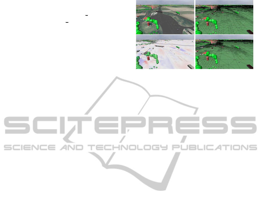
Figure 3: First row: unfiltered height data of a motorway,
last row: filter (4) applied with ε = 0.2 m and δ = 4.0 m
where height deviations are marked with colors in left pic-
ture: The bigger the difference, the darker the color, red
marks points where unfiltered heights are larger than filtered
heights, blue indicates the opposite.
n−1 going down to 0 then the formula starts adding
summands when encountering a first coefficient that
exceeds its threshold.
In contrast to JPEG 2000 we do not quantize
wavelet coefficients. For triangle count reduction
quantization does not appear to work as well as omis-
sion of coefficients. All non-zero coefficients of
Haar wavelets define height alterations that might
lead to additional triangles. But quantization does re-
duce storage space and transmission bandwidth, see
(Olanda et al., 2014).
5 HEURISTICS BASED LOW
PASS FILTERING
Our aim is to preserve salient structures like ramps,
surroundings of bridges, hills, and shore lines. Poly-
gons covering areas of these structures are available
from GIS data. Whereas fields can be drawn with re-
duced precision, a more detailed drawing is needed
for streets and railway lines. This section deals with
heuristics to implement context-sensitivefiltering that
takes care of such differences.
If a difference of unfiltered height and the result
of spline approximation at a point ( j,k) is less than
0.3 m, then this difference is not disturbing. The
threshold of 0.3 m is a parameter different than the
accuracy ε that is used for mesh simplification on the
basis of previously filtered heights. If the difference
exceeds 0.3 m, in certain circumstances we compute
a more specific height using low pass wavelet trans-
form. In this case, depending on terrain usage and
height of (j,k), we divide coordinates ( j, k) into three
main classes:
1. Class 1: A point ( j,k) is near to a point P, iff P
is located within a square covering 9
2
grid points
GRAPP2015-InternationalConferenceonComputerGraphicsTheoryandApplications
110
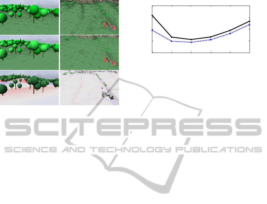
Figure 4: Triangulation based on unfiltered data (first row)
and based on non-linear filtereddata (second row) with filter
(4) and ε = 0.2 m, δ = 4.0 m. Last row shows differences
in the same manner as in Figure 3.
with ( j, k) at its center. The size of this neigh-
borhood was determined experimentally. Smaller
squares lead to poorer quality whereas larger
neighborhoods increase number of triangles un-
necessarily. In our context, high precision is re-
quired for those points ( j,k) that are near to a
point P which fulfills one of following conditions.
• P is next to a shore line of a river or lake.
• P is part of a railway embankment. If ( j,k) is
an interior point of the embankment then even
extra precision is needed to avoid non smooth
railway tracks.
• P lies within the border polygon of a bridge.
Surroundings of bridges need to be accurate
so that bridges fit into terrain. In our exam-
ple, even the finest triangle size is too coarse
to avoid gaps between bridges and their ramps.
This problem is fixed by extending bridges.
• P lies within the polygon of a street that inter-
sects at least one polygon of a bridge. Such
streets can be part of ramps.
2. Class 2: Terrain of our city model is flat apart
from some heaps and local hills. Therefore, zones
outside class 1 with unfiltered heights that dif-
fer more than a parameter δ from the heights of
spline approximation should be drawn with inter-
mediate precision. Hence heap contours remain
clearly visible. If a forest grows on a hill then even
less precision might be needed as trees hide the
ground. In our example, hilly terrain covered by
trees is limited, so that special treatment of forests
does not improve triangle count significantly. It is
not performed.
1 2 3 4 5 6
0.5
1
1.5
2
2.5
x 10
6
Figure 5: Triangle count for different numbers of spline it-
erations and accuracy levels ε, see Table 3. Broken line:
ε = 0.2 m, solid line: ε = 0.05 m (δ = 4.0 m, filter (4)).
3. Class 3: All remaining terrain can be drawn with
poor precision, i. e., heights are taken directly
from spline approximation.
We apply the simplified non-standard wavelet
transform for the grid with m·2
n
= 5·2
9
points. Low
pass filtering for points of classes 1 and 2 is done us-
ing specific sets of threshold values (t
0
,t
1
,. .. ,t
n−1
).
Height values resulting from low pass filtering re-
place heights computed by spline approximation only
if their distance to spline heights exceeds 0.3 m (less
can’t be seen).
For δ = 4 m good looking results were obtained
with threshold values from Table 1. We determined
the values experimentally. Instead, one could define
a distance measure between exact and filtered heights
(for example an L
2
distance) together with separate
local error bounds for areas of class 1 and class 2 as
constraints. Then separately for both classes, varia-
tion of thresholds can yield a set of values for which
the number of triangles becomes minimal.
Our data set contains an error where a hole ap-
pears in the middle of the harbor - probably an artifact
from a ship. Generally, heights of grid points within
polygons defining areas of water need to be constant,
because water surfaces should be flat. Linear spline
approximation and wavelet filtering do not guarantee
this outcome. This is achieved by assigning an av-
erage value to all grid points of water polygons in a
post-processing step.
6 RESULTS
We count triangles but we do not present a global
measure for quality of filtered terrain. Because we al-
low to over-simplifyareas that are uncritical for visual
impressions, measures like scene-wide L
2
metrics that
involve only height differences between filtered and
unfiltered heights are not sufficient. A comparison of
contour lines as done in (Bjørke and Nilsen, 2003)
Context-sensitiveFilteringofTerrainDatabasedonMultiScaleAnalysis
111
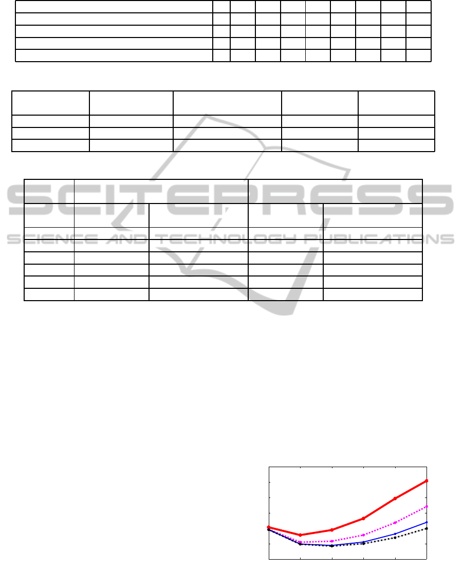
Table 1: Thresholds.
coefficient 0 1 2 3 4 5 6 7 8
class 1 0 0.1 0.1 0.2 0.2 0.2 0.3 0.3 0.4
class 1, inner points of railway embankments 0 0.1 0.1 0.1 0.1 0.1 0.1 0.1 0.1
class 2 0 0.1 0.2 0.2 0.3 0.4 0.5 0.5 0.5
class 2, forest 0 0.1 0.2 0.2 0.3 20 20 20 20
Table 2: Triangle count for δ = 4 m and three iterations of spline approximation.
triangulation triangles test data triangles spline approx. triangles, detail triangles. detail
accuracy level ε (no filtering) with unfiltered detail filtered with (3) filtered with (4)
0.2 m 2901422 1221938 962012 940214
0.1 m 4564400 1405856 1046510 1035626
0.05 m 6144422 1434602 1067888 1058636
Table 3: Influence of spline approximation on triangle count for δ = 4 m and wavelet filter (4), see Figure5.
accuracy level ε = 0.05 m accuracy level ε = 0.2 m
6144422 triangles without compression 2901422 triangles without compression
spline triangles spline triangles triangles spline triangles
iterations approximation filtered detail approximation filtered detail
1 1820300 2081120 1201376 1450412
2 544388 1158722 420140 984206
3 170210 1058636 135488 940214
4 48218 1165586 44372 1049498
5 12422 1444874 12308 1312340
6 3164 1838468 3140 1690142
might be a better tool but it lacks the ability to distin-
guish between “important” and “unimportant”.
Table 2 shows numbers of triangles in our case
study. Last two columns correspond to results of fil-
tering as described. Compression rates up to a fac-
tor of 5.8 can be reached. We have added the mid-
dle column in order to demonstrate positive effects of
low pass Haar wavelet filtering of detailed areas. It
shows triangle count when using exact heights instead
of heights resulting from wavelet filtering of points
belonging to class 1 and 2. Heights of all other points
still are taken from spline approximation. The com-
parison of the two filter variants (3) and (4) shows that
(4) produces slightly better results. That is no surprise
as highest non-zero coefficients determine size of tri-
angles. Non-zero coefficients of frequencies in the
middle do not have this effect.
Finally, we have to determine a good value for the
number of iterations of spline approximation. This
number in turn depends on the rendering of detailed
areas. Too many iterations lead to larger areas where
height deviations exceed δ. The number of triangles
saved through spline approximation then is outnum-
bered by the amount of additional triangles needed to
show details. On the other hand, too few iterations
generate a too detailed spline approximation and too
many triangles. Analysis of detailed areas then be-
comes obsolete. In our setting, for δ = 4 m the low-
est triangle count is obtained with three iterations, see
Table 3 and Figure 5. The smaller δ the larger are
areas of class 2 and the less iterations of spline ap-
proximation can be used for simplification. How δ
influences the number of spline approximations and
triangle count is shown in Table 4 and Figure 6.
With respect to different landscapes, the outcome
of our approach to filtering is shown in Figures 3 and
4.
1 2 3 4 5 6
0.5
1
1.5
2
2.5
3
3.5
x 10
6
Figure 6: Triangle count depending on iterations of spline
approximation for different height parameters δ (filter (4),
ε = 0.2 m), see Table 4. Thick solid line: δ = 1 m, dashed
line: δ = 2 m, thin solid line: δ = 4 m, dash-dot line: δ = 6
m.
GRAPP2015-InternationalConferenceonComputerGraphicsTheoryandApplications
112

Table 4: Triangle count depending on iterations of spline approximation for different height parameters δ (filter (4), ε = 0.2
m), see Figure 6.
iterations → 1 2 3 4 5 6
δ = 1.0 1529450 1274276 1440734 1813544 2460890 3038612
δ = 2.0 1458482 1044968 1075772 1275776 1676342 2203256
δ = 4.0 1450412 984206 940214 1049498 1312340 1690142
δ = 6.0 1450058 978740 917552 995828 1190306 1489028
7 CONCLUSIONS AND FUTURE
WORK
Whereas the MP3 algorithm compresses music data
by utilizing a psychoacoustic model that defines ac-
curacy of coefficients of a discrete cosine transform,
we follow a similar but more elementary approach to
reduce triangle count: Visually less important areas
are lossy compressed by applying a continuous best
spline approximation. More important areas are low
pass filtered with a wavelet transform. Thresholds for
wavelet coefficients depend on rules that take ground
usage (cadastre data) and height differences into ac-
count. This is our “psycho visual” model. Results
are promising. However, it should be investigated if
an even better quality can be obtained by additional
smoothing of certain surfaces like streets. Future
work is required to explore the method in connection
with other sets of terrain data in order to see whether
experimentally determined thresholds still work well.
The mesh simplification algorithm of Section 2 has
been chosen for simplicity. Further work is needed
to evaluate the filtering technique as a pre-processing
step that generates input for established simplification
methods.
REFERENCES
Bjørke, J. and Nilsen, S. (2003). Wavelets applied to simpli-
fication of digital terrain models. International Jour-
nal of Geographical Information Science,17:601-621.
Bruun, B. and Nilsen, S. (2003). Wavelet representation
of large digital terrain models. Computers & Geo-
sciences, 29:695–703.
Garland, M. and Heckbert, P. (1997). Surface simplifica-
tion using quadric error metrics. In Proc. 24th An-
nual Conference on Computer Graphics and Interac-
tive Techniques, SIGGRAPH ’97, pages 209–216.
Hu, H., Ding, Y., Zhu, Q., Wu, B., Lin, H., Du, Z., Zhang,
Y., and Zhang, Y. (2014). An adaptive surface filter
for airborne laser scanning point clouds by means of
regularization and bending energy. ISPRS Journal of
Photogrammetry and Remote Sensing, 92:98–111.
Kalbermatten, M. (2010). Multiscale analysis of high res-
olution digital elevation models using the wavelet
transform. EPFL Lausanne, Lausanne.
Kopp, M. and Purgathofer, W. (1998). Interleaved dimen-
sion decomposition: A new decomposition method
for wavelets and its application to computer graph-
ics. In 2nd International Conference in Central Eu-
rope on Computer Graphics and Visualisation, pages
192–199.
Losasso, F. and Hoppe, H. (2004). Geometry clipmaps: Ter-
rain rendering using nested regular grids. ACM Trans.
Graph., 23(3):769–776.
Mahler, E. (2001). Scale-Dependent Filtering of High Reso-
lution Digital Terrain Models in the Wavelet Domain.
University of Zurich, Zurich.
Mocanu, B., Tapu, R., Petrescu, T., and Tapu, E. (2011). An
experimental evaluation of 3d mesh decimation tech-
niques. In International Symposium on Signals, Cir-
cuits and Systems, pages 1–4.
Mooney, D. and Swift, R. (1999). A Course in Mathe-
matical Modeling. The Mathematical Association of
America, Washington D.C.
Olanda, R., P´erez, M., Ordu˜na, J., and Rueda, S. (2014).
Terrain data compression using wavelet-tiled pyra-
mids for online 3d terrain visualization. Interna-
tional Journal of Geographical Information Science,
28:407–425.
Silva, F. and Gomes, A. (2004). Normal-based simplifica-
tion algorithm for meshes. In Proc. Theory and Prac-
tice of Computer Graphics(TPCG 04), pages 211-218.
Strollnitz, E., DeRose, T., and Salesin, D. (1995). Wavelets
for computer graphics: a primer, part 1. IEEE Com-
puter Graphics and Applications, 15:77–84.
Vu, T. and Tokunaga, M. (2004). Filtering airborne laser
scanner data: A wavelet-based clustering method.
Photogrammetric Engineering & Remote Sensing,
70:1267–1274.
Wei, H. and Bartels, M. (2006). Unsupervised segmenta-
tion using gabor wavelets and statistical features in li-
dar data analysis. In 18th International Conference on
Pattern Recognition, pages 667–670.
Wiman, H. and Yuchu, Q. (2009). Fast compression and
access of lidar point clouds using wavelets. In Urban
Remote Sensing Event, pages 1–6.
W¨unsche, B. (1998). A Survey and Evaluation of Mesh Re-
duction Techniques. University of Auckland, Auck-
land.
Xu, L., Yang, Y., Jiang, B., and Li, J. (2007). Ground extrac-
tion from airborne laser data based on wavelet analy-
sis. In Proc. MIPPR/SPIE.
Context-sensitiveFilteringofTerrainDatabasedonMultiScaleAnalysis
113
