Single-frame Image Denoising and Inpainting Using Gaussian Mixtures
Afonso M. A. M. Teodoro
1,3
, Mariana S. C. Almeida
2,3
and M
´
ario A. T. Figueiredo
1,3
1
Instituto Superior T
´
ecnico, Universidade de Lisboa, Lisboa, Portugal
2
Priberam Labs, Lisboa, Portugal
3
Instituto de Telecomunicac¸
˜
oes, Lisboa, Portugal
Keywords:
Image Denoising, Image Inpainting, Gaussian Mixtures, Patch-based Methods, Expectation-maximization.
Abstract:
This paper proposes a patch-based method to address two of the core problems in image processing: denoising
and inpainting. The approach is based on a Gaussian mixture model estimated exclusively from the observed
image via the expectation-maximization algorithm, based on which the minimum mean squared error estimate
is computed in closed form. The results show that this simple method is able to perform on the same level as
other state-of-the-art algorithms.
1 INTRODUCTION
Denoising and inpainting are two core image process-
ing problems, with applications in digital photogra-
phy, medical and astronomical imaging, and many
others areas. As the name implies, denoising aims at
removing noise from an observed noisy image, while
the objective of painting is to estimate missing im-
age pixels. Both denoising and inpainting are inverse
problems: the goal is to infer an underlying image
from incomplete/imperfect observations thereof.
Both in inpainting and denoising, the observed im-
age y is modeled as
y = H x + n, (1)
where x is the unknown image and n is usually taken
to be a sample of white Gaussian noise, with zero
mean and variance σ
2
. In denoising, matrix H is sim-
ply an identity matrix I, while in inpaiting it contains
a subset of the rows of I, accounting for the loss of
pixels. The variance σ
2
may be assumed known, as
there are efficient and accurate techniques to estimate
it from the noisy data itself (Liu et al., 2012).
Most (if not all) state-of-the-art image denoising
methods belong to a family known as “patch-based”,
where the image is processed on a patch by patch
fashion. Several patch-based methods work by find-
ing a sparse representation of the patches, either in a
transform domain (Dabov et al., 2007) or on a learned
This work was partially supported by Fundac¸
˜
ao para
a Ci
ˆ
encia e Tecnologia, grants PEst-OE/EEI/LA0008/2013
and PTDC/EEI-PRO/1470/2012.
dictionary (Aharon et al., 2006; Elad and Aharon,
2006; Elad et al., 2010), while others search the im-
age for similar patches and combine them (Buades
et al., 2006). Finally, some methods use probabilis-
tic patch models based on Gaussian mixtures (Zoran
and Weiss, 2012; Yu et al., 2012).
There are many (in fact, too many to review in this
paper) approaches to inpaiting, ranging from methods
that smoothly propagate the image intensities from
the observed pixels to the missing ones, to dictionary-
based methods. Recent examples include the work of
Ram et al. (2013), who propose rearranging the im-
age patches so that the distance between them is the
shortest possible and then interpolate the missing pix-
els, and Zhou et al. (2012), who developed a nonpara-
metric Bayesian method for learning a dictionary that
is able to sparsely represent image patches.
In this paper, we propose a GMM-based method
that yields patch-based minimum mean squared er-
ror (MMSE) estimates, and which can handle both
denoising and inpaiting. Although GMM have been
used before for image denoising and inpaiting, our
proposal has several novel features. Unlike the ap-
proach of Yu et al. (2012), we estimate the GMM
parameters from the observed data using an exact
expectation-maximization (EM) algorithm and per-
form exact MMSE patch estimation. Unlike the
method of Zoran and Weiss (2012), ours estimates the
GMM parameters directly from the observed image
(rather than from a collection of clean patches) and
deals with both densoising and inpainting. Unlike the
proposal of Cao et al. (2008), our method also han-
283
Teodoro A., Almeida M. and Figueiredo M..
Single-frame Image Denoising and Inpainting Using Gaussian Mixtures.
DOI: 10.5220/0005256502830288
In Proceedings of the International Conference on Pattern Recognition Applications and Methods (ICPRAM-2015), pages 283-288
ISBN: 978-989-758-077-2
Copyright
c
 2015 SCITEPRESS (Science and Technology Publications, Lda.)

dles inpainting and corrects a technical flaw in their
method (details below).
2 BUILDING BLOCKS
2.1 MMSE Estimation
Let x in (1) now be one of the image patches. As is
well known from Bayesian estimation theory, the op-
timal (in the minimum mean squared error – MMSE
– sense) estimate of x is the posterior expectation,
ˆ
x = E[x | y] =
Z
x
p
Y |X
(y | x) p
X
(x)
p
Y
(y)
dx, (2)
where p
Y |X
(y | x) = N (y; H x,σ
2
I) (with N (·; µ,Σ)
denoting a Gaussian density of mean µ and covariance
Σ), resulting from the Gaussian white noise model,
and p
X
(x) is a prior density on the clean patch. It has
been argued that the state-of-the-art performance of
patch-based methods is due to the fact that they imple-
ment (or approximate) the MMSE estimate (Chatter-
jee and Milanfar, 2012). Of course, the quality of the
MMSE estimate depends critically on the adequacy
of the prior; however, the choice of prior should take
into account the (computational) difficulty in comput-
ing (2).
2.2 MMSE Estimation with GMM Prior
GMM priors have the important feature that the
MMSE estimate has a simple closed form expres-
sion, due to the fact that a GMM is a conjugate
prior for a Gaussian observation model (Bernardo
and Smith, 1994). Furthermore, it has been recently
shown that Gaussian mixtures are excellent models
for clean patches of natural images (Zoran and Weiss,
2012); but while those authors estimate the GMM pa-
rameters from a collection of clean image patches, we
show below that it is also possible to estimate them
from the noisy image itself, and still obtain competi-
tive results. Mathematically, a GMM is given by
p
X
(x | φ) =
k
∑
i=1
α
i
N (x;µ
i
,C
i
), (3)
where µ
i
and C
i
are the mean and covariance ma-
trix of the i − th component, respectively, α
i
is its
probability (of course, α
i
≥ 0 and
∑
k
i=1
α
i
= 1), and
φ = {µ
i
,C
i
,α
i
, i = 1, ...,k}.
The combination of the Gaussian observa-
tion model (likelihood function) p
Y |X
(y | x) =
N (y; H x, σ
2
I) with the GMM prior (3) allows ob-
taining the MMSE estimate in closed form (which is
a classical result in Bayesian estimation theory),
ˆ
x(y) = E[x|y] =
k
∑
i=1
β
i
(y) ν
i
(y), (4)
where
β
i
(y) =
α
i
N

y; Hµ
i
,HC
i
H
T
+ σ
2
I

k
∑
j=1
α
j
N

y; Hµ
j
,HC
j
H
T
+ σ
2
I

(5)
also satisfy β
i
(y) ≥ 0 and
∑
k
i=1
β
i
(y) = 1 (notice that
the denominator in (5) is simply p
Y
(y|φ)), and
ν
i
(y) = P
i

C
−1
i
µ
i
+
1
σ
2
H
T
y

, (6)
P
i
=

C
−1
i
+
1
σ
2
H
T
H

−1
. (7)
In fact, the posterior p
X|Y
(x|y) is itself a GMM,
p
X|Y
(x|y) =
k
∑
i=1
β
i
(y) N (x; ν
i
(y),P
i
), (8)
(from which (4) results trivially), where the weights
and the means depend on the observed y, although
the component posterior covariances do not.
Finally, from (8), it is also possible to obtain the
global posterior covariance, from its definition:
cov[x|y] = E[x x
T
|y] − E[x|y] E[x|y]
T
(9)
=
k
∑
i=1
β
i
(y)

ν
i
(y)ν
i
(y)
T
+ P
i

−
ˆ
x(y)
ˆ
x(y)
T
.
2.3 Estimating the Gaussian Mixture
There are two alternatives to estimate φ, the vector of
parameters of the prior (3), from data: it may be pre-
viously estimated from a collection of clean patches
(Zoran and Weiss, 2012); it may be estimated from
the patches of the observed data itself, which is the
approach herein proposed.
Let Y = {y
1
,...,y
N
} be the set of observations
corresponding to the set of image patches X =
{x
1
,...,x
N
}, where each y
i
is related to the corre-
sponding x
i
via an observation model of the form
(1): x
i
= H
i
x
i
+ n
i
. In the (simpler) denoising case,
H
i
= I, and the maximum likelihood estimate of φ =
{α
j
,µ
j
,C
j
, j = 1, ...,k} is given by
b
φ
ML
= argmax
φ
N
∑
i=1
log
k
∑
j=1
α
j
N

y
i
; µ
j
,C
j
+ σ
2
I

.
(10)
As is well known,
b
φ
ML
cannot be computed in closed
form, but it can be obtained efficiently using the
expectation-maximization (EM) algorithm (Dempster
et al., 1977), (Figueiredo and Jain, 2002).
ICPRAM2015-InternationalConferenceonPatternRecognitionApplicationsandMethods
284

The specific form of the EM algorithm for this
problem is almost identical to that of a standard Gaus-
sian mixture; namely, the E-step is precisely the same
as for a standard GMM and amounts to computing
w
i j
=
b
α
j
N

y
i
;
b
µ
j
,
b
C
j
+ σ
2
I

, w
i j
=
w
i j
∑
k
l=1
w
il
(11)
where
b
α
j
,
b
µ
j
,
b
C
j
, for j = 1,...,k, are the current pa-
rameter estimates.
In the M-step, the update equations for the α
j
and
µ
j
parameters are the same as for a standard GMM,
b
α
j
←
1
N
N
∑
i=1
w
i, j
,
b
µ
j
←
1
N
b
α
j
N
∑
i=1
w
i, j
µ
j
, (12)
whereas the covariances are updated according to
b
C
j
← V
j

Λ
j
− σ
2
I

+
V
T
j
, (13)
where Λ
j
is the diagonal matrix with the eigenvalues
of the matrix
D
j
=
1
N
b
α
j
N
∑
i=1
w
i j
(y
i
−
b
µ
j
)(y
i
−
b
µ
j
)
T
,
and V
j
is the matrix with the corresponding eigen-
vectors; finally, (·)
+
denotes the element-wise appli-
cation of the positive part operator z
+
= max{z,0}.
Cao et al. (2008) also use EM to estimate the
GMM parameters from the noisy patches. However,
the covariance estimates are not computed as in (13),
but simply as D
j
− σ
2
I. As a consequence, several
covariance estimates may have negative eigenvalues
(thus being invalid), which is almost sure to happen
in cases of moderate or strong noise.
The inpainting case, which is more difficult due
to the presence of the H
i
matrices, can be seen as
the problem of estimating the parameters of a GMM,
from a collection of observations with missing en-
tries. This problem has been recently addressed by
Eirola et al. (2014), and we adapt their algorithm to
our particular parameterization of the covariance ma-
trices. We omit details for lack of space.
3 PATCH-BASED METHOD
The proposed approach follows the standard patch-
based denoising protocol using the building blocks
described in the previous section.
1. All (overlapping) patches of size p
d
× p
d
are ex-
tracted from the observed image, yielding the col-
lection of observed patches Y = {y
1
,...,y
N
}.
2. The parameters of the GMM are estimated from
Y via the EM algorithm presented in Section 2.3.
3. The MMSE estimates of all the patches are ob-
tained as described in Section 2.1, yielding the set
of estimated patches
b
X = {
b
x
1
,...,
b
x
N
}.
4. The final image estimate is assembled by putting
the patch estimates
b
X = {
b
x
1
,...,
b
x
N
} back in the
same locations from where the corresponding
noisy (or incomplete, in inpainting) patches were
extracted. Since the patches overlap, there are
several estimates of each pixel, which are stan-
dardly combined by computing a straight average.
Combining the overlapping patch estimates by
straight averaging ignores that estimates coming from
different patches may have different degrees of con-
fidence. In a Bayesian framework, this confidence is
given by the (inverse of the) posterior variance, i.e.,
the diagonal of the posterior covariance matrix in (9).
Accordingly, we combine the pixel estimates from
each patch by weighted averaging, with weights set
to the inverses of the posterior variances. The use of
variances to weight the pixel estimates was already
exploited by Dabov et al. (2007), but their method
uses patch-wise variance estimates, rather than a pos-
terior variance for each pixel in each patch. Indi-
vidual pixel variances were also used to weight the
corresponding estimates by Chatterjee and Milanfar
(2012), but they use a single Gaussian per patch.
4 FURTHER IMPROVEMENTS
4.1 Dealing with the DC Component
To decrease the number of GMM parameters to esti-
mate, it is possible to assume that all the components
have zero mean. In principle, this assumption incurs
in no loss of generality, as it is possible to center the
image by subtracting its mean. In this case, all the ex-
pressions above simplify with µ
j
= 0, for j = 1, ...,k.
Alternatively to removing the mean from the
whole input image, it is also possible to center each
patch with respect to its own mean (DC component).
In this case, the processing chain starts by comput-
ing, storing, and subtracting the average from each
patch; after the patch estimates are obtained, these
means are added back to each patch before the final
image assembling step. Under the assumption of ad-
ditive white Gaussian (AWGN), the patch-wise aver-
aging reduces the noise variance by a factor of p
d
× p
d
(the number of samples in each patch). Consequently,
the set of observed patch means can be seen as result-
ing from the true patch means via the contamination
with zero-mean Gaussian noise with variance σ
2
/p
2
d
.
Single-frameImageDenoisingandInpaintingUsingGaussianMixtures
285

Table 1: PSNR comparison on gray-level image denoising of the following methods: BM3D (Dabov et al., 2007); K-SVD
(Elad and Aharon, 2006); basic proposed algorithm (Section 3); improved proposed algorithm (Sections 4.1 and 4.2).
σ
Lena (512 × 512) Cameraman (256 × 256) House (256 × 256)
BM3D K-SVD Basic Improved BM3D K-SVD Basic Improved BM3D K-SVD Basic Improved
5 38.72 38.53 38.86 38.86 38.29 37.97 38.57 38.58 39.83 39.47 39.92 39.94
10 35.93 35.55 35.88 35.88 34.18 33.76 34.44 34.49 36.61 36.05 36.58 36.62
15 34.27 33.74 34.11 34.11 31.91 31.54 32.15 32.21 34.94 34.41 34.65 34.69
20 33.05 32.40 32.83 32.84 30.48 30.07 30.64 30.70 33.77 33.21 33.34 33.46
25 32.08 31.34 31.81 31.82 29.45 28.94 29.50 29.58 32.86 32.21 32.34 32.49
30 31.26 30.46 30.99 31.00 28.64 28.12 28.58 28.66 32.09 31.25 31.44 31.66
Table 2: PSNR on gray-level image inpainting for different data ratios and methods: BP (Zhou et al., 2012), SOP (Ram et al.,
2013), our basic method, and the one using sub-images (Section 4.3).
Method
Lena (512 × 512) Cameraman (256 × 256) House (256 × 256) Barbara256 (256 × 256)
80% 50% 20% 80% 50% 20% 80% 50% 20% 80% 50% 20%
BP 41.27 36.94 31.00 34.70 28.90 24.11 43.03 38.02 30.12 41.12 35.60 26.87
SOP 43.01 37.43 31.94 36.19 30.71 25.13 44.34 38.77 32.60 42.25 35.97 28.98
Basic 41.91 37.22 31.25 33.74 28.85 24.11 45.20 39.30 31.71 43.90 37.11 28.05
Subimages 41.98 37.57 31.78 35.03 29.36 24.25 45.39 39.42 32.05 44.56 37.15 28.41
4.2 Dealing with Flat Patches
In a gray-scale image, a flat area is characterized by a
constant intensity level, thus with zero variance. Con-
sidering AWGN with variance σ
2
, the variance of a
flat area is approximately the same as the variance of
the noise. It has been shown empirically that treat-
ing patches that are (almost) flat separately leads to
an increase in performance (Lebrun et al., 2013); an
observed image patches is declared as flat if its sam-
ple variance falls below C σ
2
, where C is a constant
close to 1. Of course, this criterion is not foolproof; in
fact, for high values of σ
2
, it is difficult to distinguish
between flat patches and textured patches. After the
identification of the flat patches, these are denoised
simply by replacing them by their sample mean.
4.3 Dividing the Image into Sub-images
The last improvement (also used by Dabov et al.
(2007) and Ram et al. (2013)) is to divide the noisy
image into a set of smaller (but much larger than
the patches) sub-images and treat them independently
from each other. To avoid artifacts at the boundaries,
the sub-images should have a small amount of over-
lap, and the final image obtained by averaging the es-
timates coming from each sub-image. This strategy
allows using different patch sizes and different num-
bers of mixture components on each sub-image, al-
lowing a better adaptation of the model to different
areas of the image. Finally, dealing separately with
each sub-image reduces the memory requirements of
the algorithm and allows a straightforward, yet not
ideal, parallel implementation.
5 RESULTS AND DISCUSSION
5.1 Denoising
Table 1 presents denoising results obtained with the
basic version of the proposed method described in
Section 3, a version with the improvements presented
in Sections 4.1 and 4.2, as well as the results ob-
tained with the well known BM3D (Dabov et al.,
2007) and K-SVD (Elad and Aharon, 2006) algo-
rithms. These two reference methods were chosen
because they are state-of-the-art patch-based methods
with publicly available implementations. In the re-
sults reported in Table 1, the patch size p
d
and k were
chosen to yield the best results.
We performed several experiments to study the
impact of those parameters in the denoising perfor-
mance of the method: for each input image and noise
variance, both p
d
and k were swept from 3 to 12 and
from 10 to 60 (in steps of 5), respectively. Figure 1 re-
ports some of those experiments, the results of which
provide some insight on the behaviour of the method.
As is clear by comparing the plots in Figure 1 (a) and
(b)), the optimal patch size is larger when the noise is
stronger, which is a natural result; in fact, using larger
(overlapping) patches means having more estimates
of each pixel, thus a more aggressive denoising. On
the other hand, the mixture should have enough com-
ponents to be sufficiently expressive, but the results
ICPRAM2015-InternationalConferenceonPatternRecognitionApplicationsandMethods
286

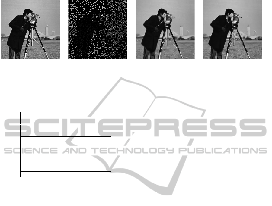
(a) (b) (c) (d)
Figure 2: Denoising: (a) original image; (b) noisy image (σ = 30, PSNR = 18.59dB); (c) BM3D (Dabov et al., 2007); (d)
Proposed.
4 6 8 10 12
38
38.1
38.2
38.3
38.4
38.5
pd
PSNR (dB)
Cameraman 256x256, σ =5
K = 10
K = 30
K = 50
4 6 8 10 12
27
27.5
28
28.5
pd
PSNR (dB)
Cameraman 256x256, σ =30
K = 10
K = 30
K = 50
(a) (b)
4 6 8 10 12
28.5
29
29.5
30
30.5
pd
PSNR (dB)
Lena 512x512, σ =30
K = 30
4 6 8 10 12
28.5
29
29.5
30
30.5
31
pd
PSNR (dB)
House 256x256, σ =30
K = 30
(c) (d)
Figure 1: PSNR as a function of p
d
and k: (a–b) varying
p
d
, with k ∈ {10,30,50}, for σ = 5 and σ = 30; (c) varying
p
d
on a larger image, for K = 30,σ = 30; (d) Varying p
d
on
a flatter input image, K = 30,σ = 30.
(specially with strong noise) depend weakly on k (no-
tice that the range of the vertical axis in Figure 1 (a)
is only roughly 0.5 dB). For higher resolution images
(Figure 1 (c)), the method performs better with larger
patches, arguably due to the sheer number of pixels.
Finally, on images with many flat patches (Figure 1
(d)) relatively larger values of p
d
yield better results,
in agreement with the fact that for larger patches the
DC component can be estimated more precisely.
These dependencies, although not very strong, are
a downside of the proposed method (and of many
other patch-based methods) and strategies to make the
algorithm more adaptive should be developed. For ex-
ample, the number of GMM components may be es-
timated directly from the data, e.g., using the method
proposed by Figueiredo and Jain (2002). Of course,
there is no guarantee that the criterion therein used
to select the number of components also yields the
best denoising results when the estimated mixture is
used for that purpose. Nevertheless, the obtained re-
sults compete with other state-of-the-art algorithms,
specially for lower noise variances (the most useful
range in practice), and the modifications are able to
slightly increase the output PSNR.
Finally, Figure 2 illustrates the visual quality of
the obtained denoised images, in comparison with the
BM3D method (Dabov et al., 2007). In this case,
BM3D produces a slightly more appealing denoised
image in the flatter regions.
5.2 Inpainting
For inpainting, we focused on finding the parameters
leading to the best results as the data ratio decreases.
An aspect worth stressing is that the patches should
be large enough to allow each of them to have a sig-
nificant fraction of known pixels. Table 2 shows the
experimental results on pure inpainting (σ = 0). The
reference methods (BP (Zhou et al., 2012) and SOP
(Ram et al., 2013)) were chosen because they are
patch-based, state-of-the-art, and publicly available.
Figure 3 exemplifies the visual quality of the output;
although in terms of PSNR the proposed method is
behind SOP, our estimate is visually better. Table 3
shows results of simultaneous inpainting and denois-
ing, for the test image used by Zhou et al. (2012). In
both tables (2 and 3), the results were obtained with
p
d
= 10 and k = 25. The proposed method is able to
obtain state-of-the-art results, not only in inpainting
but also on simultaneous inpainting and denoising.
6 CONCLUSIONS
We have presented a patch-based method that han-
dles both image denoising and inpainting, based on a
Gaussian mixture model learned directly from the ob-
served image and using the exact expression for the
minimum mean squared error estimate. The proposed
formulation also yields the posterior variances of each
Single-frameImageDenoisingandInpaintingUsingGaussianMixtures
287

(a) (b) (c) (d)
Figure 3: Inpainting: (a) original image; (b) corrupted image (80% missing pixels; PSNR = 6.56dB); (c) SOP (Ram et al.,
2013); (d) Proposed.
Table 3: Simultaneous inpainting and denoising results in
terms of PSNR - Methods: BP (Zhou et al., 2012); Basic
algorithm (Section 2); Subimages framework (Section 4.3).
σ Data Ratio
Barbara256 (256 × 256)
BP Basic Subimages
5
80% 36.80 37.16 37.25
50% 33.61 33.82 34.02
20% 26.73 27.45 28.04
15
80% 31.24 31.63 31.79
50% 29.31 28.92 29.14
20% 25.17 25.24 25.52
25
80% 28.40 28.92 29.05
50% 26.79 26.46 26.61
20% 23.49 23.53 23.74
pixel estimate, which provide the optimal weights to
combine the patches when assembling the final im-
age. The experimental results shows that the proposed
method is competitive with the state-of-the-art.
REFERENCES
Aharon, M., Elad, M., and Bruckstein, A. (2006). K-SVD:
an algorithm for designing overcomplete dictionaries
for sparse representation. IEEE Trans. on Signal Pro-
cessing, 54:4311–4322.
Bernardo, J. and Smith, A. (1994). Bayesian Theory. Wiley.
Buades, A., Coll, B., and Morel, J. M. (2006). A review of
image denoising methods, with a new one. Multiscale
Modeling and Simulation, 4:490–530.
Cao, Y., Luo, Y., and Yang, S. (2008). Image denoising with
Gaussian mixture model. In Congress on Image and
Signal Proc., vol. 3, pages 339–343.
Chatterjee, P. and Milanfar, P. (2012). Patch-based near-
pptimal image denoising. IEEE Trans. Image Proc.,
21:1635–1649.
Dabov, K., Foi, A., Katkovnik, V., and Egiazarian, K.
(2007). Image denoising by sparse 3D transform-
domain collaborative filtering. IEEE Trans. Image
Proc., 16(8):2080–2095.
Dempster, A. P., Laird, N. M., and Rubin, D. B. (1977).
Maximum likelihood from incomplete data via the
EM algorithm. Journal of the Royal Statistical So-
ciety, Series B, 39(1):1–38.
Eirola, E., Lendasse, A., Vandewalle, V., and Biernacki, C.
(2014). Mixture of Gaussians for distance estimation
with missing data. Neurocomputing, 131:32–42.
Elad, M. and Aharon, M. (2006). Image denoising via
sparse and redundant representations over learned dic-
tionaries. IEEE Trans. Image Proc., 15:3736–3745.
Elad, M., Figueiredo, M., and Ma, Y. (2010). On the role
of sparse and redundant representations in image pro-
cessing. Proceedings of the IEEE, 98:972–982.
Figueiredo, M. and Jain, A. K. (2002). Unsupervised learn-
ing of finite mixture models. IEEE Trans. on Pattern
Analysis and Machine Intelligence, 24:381–396.
Lebrun, M., Buades, A., and Morel, J.-M. (2013). A non-
local Bayesian image denoising algorithm. SIAM J.
Imaging Sciences, 6(3):1665–1688.
Liu, X., Tanaka, M., and Okutomi, M. (2012). Noise level
estimation using weak textured patches of a single
noisy image. In 19th IEEE International Conference
on Image Processing, 2012, pages 665–668.
Ram, I., Elad, M., and Cohen, I. (2013). Image processing
using smooth ordering of its patches. IEEE Trans. on
Image Processing, 22:2764–2774.
Yu, G., Sapiro, G., and Mallat, S. (2012). Solving inverse
problems with piecewise linear estimators: From
Gaussian mixture models to structured sparsity. IEEE
Trans. Image Processing, 21:2481–2499.
Zhou, M., Chen, H., Paisley, J., Ren, L., Li, L., Xing, Z.,
Dunson, D., Sapiro, G., and Carin, L. (2012). Non-
parametric Bayesian Dictionary Learning for Analysis
of Noisy and Incomplete Images. Image Processing,
IEEE Trans. on, 21(1):130–144.
Zoran, D. and Weiss, Y. (2012). Natural Images, Gaussian
Mixtures and Dead Leaves. In Advances in Neural In-
formation Processing Systems 25, pages 1736–1744.
ICPRAM2015-InternationalConferenceonPatternRecognitionApplicationsandMethods
288