A Linear Time Algorithm for Visualizing Knotted Structures in 3 Pages

Vitaliy Kurlin

1,2

Microsoft Research Cambridge, 21 Station Road, Cambridge CB1 2FB, U.K.

Mathematical Sciences, Durham University, Durham DH1 3LE, U.K.

Keywords:

Graph Visualization, Graph Drawing, Knot, Knotted Graph, Book Embedding, Plane Diagram, Gauss Code.

Abstract:

We introduce simple codes and fast visualization tools for knotted structures in molecules and neural networks.

Knots, links and more general knotted graphs are studied up to an ambient isotopy in Euclidean 3-space. A

knotted graph can be represented by a plane diagram or by an abstract Gauss code. First we recognize in

linear time if an abstract Gauss code represents an actual graph embedded in 3-space. Second we design a

fast algorithm for drawing any knotted graph in the 3-page book, which is a union of 3 half-planes along their

common boundary line. The running time of our drawing algorithm is linear in the length of a Gauss code

of a given graph. Three-page embeddings provide simple linear codes of knotted graphs so that the isotopy

problem for all graphs in 3-space completely reduces to a word problem in ﬁnitely presented semigroups.

1 MOTIVATION AND PROBLEMS

Knotted structures are common in nature. For exam-

ple, microscopic lines in liquid-crystals (Tkalec et al.,

2011) or Reeb graphs of complex shapes (Biasotti et

al., 2008) can be knotted. Figure 1 shows a neuron

and a microscopic scan of a chemical. These struc-

tures are usually huge and more complicated than

simple closed curves studied in classical knot theory.

Pictures of knots can be attractive for humans, but

robots would prefer a smaller form or codes represent-

ing the same knotted object. Such codes are needed

for automatic analysis, however a ﬁnal output is im-

portant to visualize. We summarize our requirements

for processing knotted structures in 3 problems.

• Modeling: ﬁnd a suitable mathematical model for

analyzing all possible knotted structures in 3-space.

• Encoding: represent any knotted structure by its

simple and small code in a computer’s memory.

• Visualization: design a fast algorithm to visualize

knotted structures represented by their abstract codes.

Figure 1: Neurons and molecules have branching points.

Our suggested model for knotted structures is a

possibly disconnected graph with branching vertices

and multiple edges that might be knotted in 3-space,

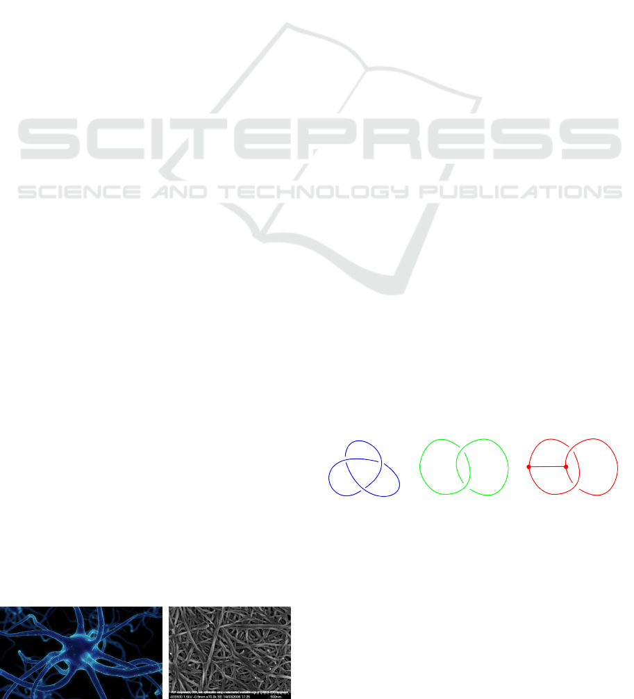
see Deﬁnition 1. For instance, any knot in 3-space is

a non-self-intersecting closed curve, which is a topo-

logical circle without any branching points.

Knots live in 3-space, but it is easier to draw their

planar projections with double crossings. Such plane

diagrams are usually represented by Gauss codes that

specify the order of overcrossings and undercrossings

along a knot. We extend classical Gauss codes of

knots to arbitrary knotted graphs in Deﬁnition 4.

Figure 2: Diagrams of the trefoil, Hopf link, knotted graph.

A random code (of a required form) may not rep-

resent a real knotted graph, because a planar draw-

ing may need extra crossings. We solve this planarity

problem for Gauss codes of knotted graphs in Theo-

rem 9. Namely, our algorithm checks if a Gauss code

is realized by an actual graph in 3-space with a linear

time complexity in the length of the given code.

Starting from any realizable Gauss code, we draw

a corresponding graph in the 3-page book, see Theo-

rem 12. This book consists of 3 half-planes attached

along their common boundary α called the spine.

Kurlin V..

A Linear Time Algorithm for Visualizing Knotted Structures in 3 Pages.

DOI: 10.5220/0005259900050016

In Proceedings of the 6th International Conference on Information Visualization Theory and Applications (IVAPP-2015), pages 5-16

ISBN: 978-989-758-088-8

 2015 SCITEPRESS (Science and Technology Publications, Lda.)

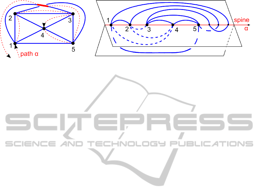
Figure 3: Straighten a red path α to build a 3-page embedding of a knotted graph K

⊂ R

from its plane diagram.

It is well-known that any graph can be topolog-

ically embedded in the 3-page book (Bernhart and

Kainen, 1979, Theorem 5.4). However, an embedded

graph may cross many times the spine of the book. It

is only known that O(|E|log |V |) spine crossings suf-

ﬁce for embedding a graph with |V | vertices and |E|

edges (Enomoto and Miyauchi, 1999).

We largely strengthen the former result by design-

ing a linear time algorithm to continuously move any

graph embedded in 3-space to a graph within 3 pages.

We review other related work throughout the paper.

Figure 3 is a high-level illustration of our fast algo-

rithm for a knotted graph K

⊂ R

. Appendix con-

tains more details on the following advantages of 3-

page embeddings over traditional plane diagrams.

• Theorem 13 encodes 3-page embeddings of all

knotted graphs by easy codes that form a semigroup.

• Theorem 14 decomposes any topological equiv-

alence between 3-page embeddings of graphs into

ﬁnitely many local relations between 3-page codes.

2 KEY CONCEPTS ON GRAPHS

A homeomorphism between spaces is a bijection that

is continuous in both directions. An embedding of one

space into another is a continuous function f : X → Y

that induces a homeomorphism between X and its im-

age f (X ) ⊂ Y. We study embeddings of undirected

ﬁnite graphs, possibly disconnected and with loops or

multiple edges. The concept of a knotted graph ex-

tends the classical theory of knots to arbitrary graphs

considered up to isotopy in 3-space R

Deﬁnition 1. A knotted graph G ⊂ R

is an embed-

ding of a ﬁnite graph G. An ambient isotopy between

knotted graphs G, H ⊂ R

is a continuous family of

homeomorphisms f

: R

→ R

, t ∈ [0, 1] such that

= id is the identity map on R

and f

(G) = H.

An isotopy between directed graphs is similarly

deﬁned and should respect directions of edges. If the

underlying graph G is a circle S

, then a knotted graph

is a knot. If G is a disjoint union of several circles,

then G ⊂ R

is a link. A link isotopic to a union of

disjoint circles in R

is called trivial. The simplest

non-trivial knot is the trefoil in Figure 2. The simplest

non-trivial link is the Hopf link in Figure 2.

If an ambient isotopy keeps a small neighborhood

of each vertex of a knotted graph in one moving plane,

the graph is called rigid. Rigid knotted graphs with

vertices of only degree 4 are sometimes called singu-

lar knots, because they consist of one or several cir-

cles intersecting each other at singular points.

Deﬁnition 2. A plane diagram D of a knotted graph

G ⊂ R

is the image of G under a projection R

→

from 3-space R

to a horizontal plane R

. In a

general position we assume that all intersections of

a plane diagram D are double crossings so that the

crossings and the projections of all vertices of G are

distinct. For each crossing of D, we specify one of two

intersecting arcs that crosses over another arc.

The key problem in knot theory is to efﬁciently

classify knots and graphs up to ambient isotopy. The

ﬁrst natural step is to reduce the dimension from 3 to

2. Any isotopy of knotted graphs can be realized by

ﬁnitely many moves on plane diagrams. The follow-

ing result extends Reidemeister’s theorem for knots.

Theorem 3. (Kauffman, 1989) Two plane diagrams

represent isotopic knotted graphs in 3-space R

if and

only if the diagrams can be obtained from each other

by an isotopy in R

and ﬁnitely many Reidemeister

moves in Figure 4. (The move R5 is only for rigid

graphs, the move R5

is only for non-rigid graphs.)

The move R4 is shown only for a degree 4 vertex,

moves for other degrees are similar. The move R5

turns a small neighborhood of a vertex in the plane

upside down. So a cyclic order of edges at vertices is

preserved in rigid graphs. The move R5

can arbitrar-

ily reorder all edges at a vertex. Theorem 3 formally

includes all symmetric images of moves in Figure 4.

The Reidemeister moves or their analogs on Gauss

codes are not local as they involve distant parts of a

IVAPP2015-InternationalConferenceonInformationVisualizationTheoryandApplications

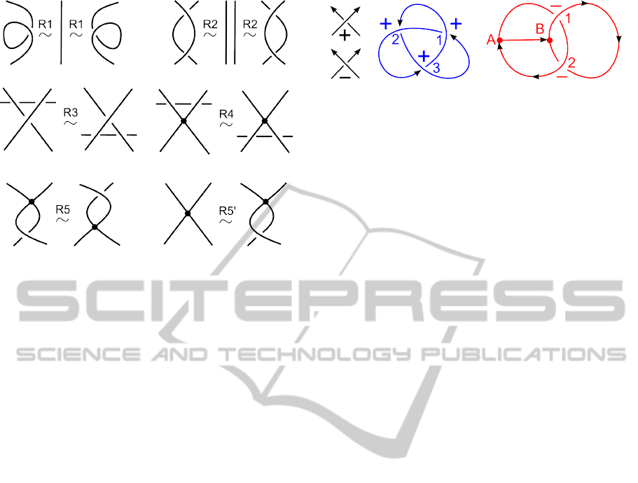
Figure 4: Reidemeister moves on diagrams of graphs.

graph or a Gauss code. This non-locality is a key ob-

stacle for simplifying codes of knots. That is why

we later consider 3-page embeddings that allow only

ﬁnitely many local moves, see Theorem 12.

3 CODES OF KNOTTED GRAPHS

A standard way to encode a plane diagram of a knot is

to write down labels of crossings in a Gauss code. The

Gauss code of a link has several words corresponding

to all link components. We extend this classical con-

cept to arbitrary knotted graphs G ⊂ R

. If a compo-

nent of G is a circle without vertices, we add a base

point (a degree 2 vertex) to this circle.

Deﬁnition 4. Let D ⊂ R

be a plane diagram of a

knotted graph G with vertices A, B, C, . . . We ﬁx direc-

tions of all edges of G and arbitrarily label all cross-

ings of D by 1, 2, . . . , n. Then each crossing of D has

the sign locally deﬁned in Figure 5. The Gauss code

of D consists of all words W

associated to directed

edges from a vertex A to a vertex B as follows:

• the word W

starts with A, ﬁnishes with B and has

the labels of all crossings in the directed edge AB;

• if AB goes under another edge at a crossing i with a

sign ε ∈ {±} as in Figure 5, we add the superscript ε

to i and get the symbol i

with the sign ε in W

The neighbors (vertices or crossings) of each vertex A

are clockwisely ordered in R

, so the code also spec-

iﬁes a cyclic order of all symbols adjacent to A.

If a graph G is a knot, Deﬁnition 4 requires at least

one degree 2 vertex (a base point) on G. For simplic-

ity, we may ignore degree 2 vertices in this case and

consider the corresponding single word cyclically.

Figure 5: Local rules for signs of crossings with examples.

In Figure 5 the diagram of the blue trefoil has

the cyclic Gauss code 12

. The diagram

of the red knotted graph has the Gauss code W =

{AB, A1

−

2A, B12

−

B} with the cyclic orders of neigh-

bors at both vertices A : (B, 2, 1

−

), B : (A, 1, 2

−

A Gauss code of any undirected graph depends

on a choice of extra degree 2 vertices, directions of

edges, an order of crossings. If a plane diagram of a

knotted graph corresponds to a Gauss code, then this

diagram is unique up to isotopy in the plane. We give

an explicit construction in the proof of Theorem 9.

Here is a naive approach to drawing a plane dia-

gram represented by a Gauss-like code W . We can

put vertices A, B, C, . . . and crossings 1, 2, . . . , n at ar-

bitrary points in R

. Since the code W speciﬁes the

cyclic order of edges at each vertex A in Deﬁnition 4,

we may draw short arcs around A in a correct cyclic

order. Now we should connect all vertices and cross-

ings that have adjacent positions in the code W by

continuous non-intersecting arcs in the plane.

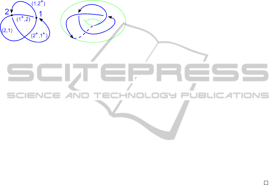
The last step fails for the word 12

2 that does

not encode any plane diagram. Indeed, if we try to

draw a closed curve with 2 self-intersections as re-

quired by 12

2, we have to add a 3rd intersection

(a virtual crossing) to make the curve closed. This ob-

stacle can be resolved if we draw a diagram on a torus

as in Figure 6, because we can hide a virtual crossing

by adding a handle. Another approach is to embrace

virtual crossings, which has led to virtual knots.

If we study properly embedded graphs, we need to

recognize planarity of Gauss codes, namely determine

if a Gauss code represents a plane diagram of a knot-

ted graph. So we ﬁrst introduce abstract Gauss codes

in Deﬁnition 5 and then recognize their planarity in

the general case of knotted graphs in Theorem 9.

Deﬁnition 5. Let the alphabet consist of m letters

A, B, C, . . . and 3n symbols i, i

, i

−

for i = 1, . . . , n. An

abstract Gauss code is a set of words such that

• the ﬁrst and last symbols of each word are letters,

• the set of symbols in all words (apart from the initial

and ﬁnal letters) contains, for each i = 1, . . . , n, the

symbol i and exactly one symbol from the pair i

, i

−

Each of the m letters deﬁnes a cyclic order of all sym-

bols adjacent to this letter. The length |W | is the total

ALinearTimeAlgorithmforVisualizingKnottedStructuresin3Pages

length of all words minus the number of words.

The Gauss code of any plane diagram of a knot-

ted graph G from Deﬁnition 4 satisﬁes the conditions

above. Indeed, the letters A, B, C, . . . denote (projec-

tions of) vertices of G. Then every edge contains

crossings labeled by i, i

or i

−

for i = 1, . . . , n.

Figure 6: A diagram with 1 virtual, 2 usual crossings.

The clockwise order of edges around any vertex

A in the plane diagram of G in R

deﬁnes the cyclic

order of vertices and crossings adjacent to A. If a

component of G is a circle, we may remove its ver-

tices of degree 2 and write the remaining symbols as

in the cyclic code 12

of the trefoil in Fig-

ure 5. The total number of these symbols equals the

doubled number of crossings.

4 PLANARITY OF GAUSS CODES

The planarity problem is to determine whether it is

possible to draw a plane diagram represented by an

abstract Gauss code W . To avoid potential self-

intersections, we shall draw a diagram not in the

plane, but in the Gauss surface S(W ) deﬁned below.

First we introduce the abstract graph G(W ) de-

scribing the adjacency relations between symbols in

a Gauss code W . Then we attach disks to G(W ) to get

the surface S(W ) containing a required diagram with-

out self-intersections. The criterion of planarity will

check if the surface S(W ) is a topological sphere S

Deﬁnition 6. Any abstract Gauss code W with m

letters A, B, . . . and 2n symbols from {i, i

, i

−

| i =

1, . . . , n} gives rise to the Gauss graph G(W ) with

m + n vertices labeled by A, B, . . . and 1, 2, . . . , n.

We connect vertices p, q by a single edge in G(W )

if p, q (possibly with signs) are adjacent symbols in

W . Below when we travel along an edge from p to

q, we record our path by (p, q)

if q follows p in the

code W (in the cyclic order), otherwise by (p, q)

−

We deﬁne unoriented cycles in the graph G(W ) by

going along edges and turning at vertices according

to the following rules illustrated in Figure 7:

• if we came to one of the vertices A, B, C, . . . from

its neighbor, then we turn to the next neighbor in the

clockwise order speciﬁed in the Gauss code W ;

• at each vertex labeled by i ∈ {1, . . . , n} we turn to

the next edge by one of the rules below for a unique

possible choice of δ ∈ {+, −} and both ε ∈ {+, −}

(p, i)

→ (i

, q)

, (p, i)

−

→ (i

, q)

−δ

(p, i

)

→ (i, q)

−ε

, (p, i

−

)

→ (i, q)

We stop traversing cycles when every edge was passed

once in each direction. The Gauss surface S(W ) is

obtained from G(W ) by gluing a disk to each cycle.

The number of edges in the graph G(W ) equals

the length |W| of the code W . The rules for traversing

cycles in Deﬁnition 6 geometrically mean that at each

vertex or crossing we turn left to a unique edge and

can pass every edge exactly once in each direction.

Hence the Gauss surface of any abstract Gauss code

is a compact orientable surface without boundary.

Lemma 7. For the Gauss code W of any plane dia-

gram of a knotted graph G ⊂ R

, the Gauss surface

S(W ) is homeomorphic to a topological sphere S

Proof. We assume that the given diagram D is con-

tained in a sphere S

instead of a plane R

. Then the

Gauss graph G(W ) can be identiﬁed with the diagram

D, though G(W ) was introduced as an abstract graph

not embedded into any space. When we traverse the

cycles in D = G(W ) from Deﬁnition 6, we pass over

the boundaries of all connected components of S

−D.

Indeed, each time we turn left in the diagram D ⊂ S

according to the geometric rules in Figure 7. Hence

the Gauss surface S(W) can be identiﬁed with the

sphere S

containing the diagram D = G(W ).

Example 8. We construct the Gauss surface of the

abstract Gauss code W = 12

2, whose diagram

with one virtual crossing is in Figure 8. For simplicity,

we removed the degree 2 vertex from the circle and

consider the word 12

2 in the cyclic order.

Then 4 pairs 12

, 2

, 1

2, 21 of adjacent sym-

bols in the code W lead to the graph G(W ) whose 2

vertices with labels 1, 2 are connected by 4 edges with

labels (1, 2

), (2

, 1

), (1

, 2), (2, 1) in Figure 8.

Recall that the edges labeled by (2, 1) and (2

, 1

)

meet at a non-avoidable virtual crossing in the plane,

but the abstract graph G(W ) has only 2 vertices.

If we start traveling from the edge (1, 2

)

the same direction as in W , the next edge should

be (2, 1

)

−

by the rule (p, i

)

→ (i, q)

−ε

, where

p = 1, i = 2, ε = + uniquely determine the next sym-

bol q = 1

from the code W (going from 2 in the

opposite direction). After the second edge (2, 1

)

−

IVAPP2015-InternationalConferenceonInformationVisualizationTheoryandApplications

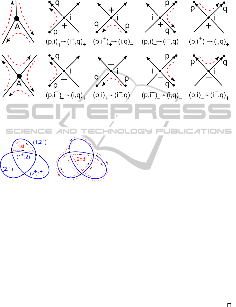
Figure 7: A geometric interpretation of the ‘turning-left’ rules for traversing cycles in the Gauss graph G(W ).

we return to the ﬁrst edge (1, 2

)

by the same rule

(p, i

)

→ (i, q)

−ε

for p = 2, i = 1, ε = −, q = 2

Figure 8: Two red dashed cycles in G(W ) for W = 12

So the 1st cycle consists of 2 edges (12

)

and (2, 1

)

−

. The 2nd cycle consists of 6

edges (1

, 2)

→ (2

, 1

)

→ (1, 2)

−

→ (2

, 1)

−

→

, 2

)

−

→ (2, 1)

. Both cycles of G(W ) are shown

by red dashed closed curves in Figure 8. The result-

ing Gauss surface S(W) with 2 vertices, 4 edges, 2

faces has the Euler characteristic χ = 2 − 4 + 2 = 0

and should be a torus as expected from Figure 6.

The Euler characteristic of a surface subdivided

by a graph with |V | vertices and |E| edges into |F|

faces (topological disks) is deﬁned as χ = |V | − |E| +

|F| and is invariant up to a homeomorphism (a bijec-

tion continuous in both directions).

Any orientable connected compact surface of a

genus g (the number of handles) and b boundary com-

ponents (circles) has χ = 2 − 2g − b ≤ 2. Hence a

sphere S

with χ(S

) = 2 is detectable by the Euler

characteristic among connected compact surfaces.

Theorem 9 extends (Kurlin, 2008, Algorithm 1.4)

from links to arbitrary knotted graphs.

Theorem 9. Given an abstract Gauss code W of a

length |W |, an algorithm of time complexity O(|W |)

can determine if the given Gauss code W represents a

plane diagram of a knotted graph G ⊂ R

Proof. The Gauss surface S(W ) of any abstract Gauss

code W contains the diagram D encoded by W due to

the geometric interpretation of the rules in Figure 7.

This surface has the maximum Euler characteristic χ

among all orientable connected compact surfaces S

that contain the diagram D and have no boundary.

Indeed, after cutting the underlying graph of the

diagram D ⊂ S, the surface S splits into several com-

ponents. The Euler characteristic of S is maximal

when all these components are disks as in the Gauss

surface. The disk has χ = 1, which is maximal among

all compact surfaces whose boundary is a circle.

To decide the planarity of W , it remains to deter-

mine if the Gauss surface S(W ) is a sphere S

, which

is detectable by the Euler characteristic χ = 2 in the

class of all orientable connected compact surfaces S

without boundary. For computing the Euler charac-

teristic χ, we use the Gauss graph G(W ), which splits

S(W ) into topological disks by Deﬁnition 6.

Namely, S(W ) has m + n vertices, |W | edges and

the number of faces equal to the number of cycles.

We count all cycles in G(W ) in time O(|W |) by a dou-

ble traversal of W according to the rules in Figure 7.

Hence in time O(|W |) we compute χ = m + n − |W | +

#(cycles) and determine if the Gauss surface S(W ) is

homeomorphic to a topological sphere S

ALinearTimeAlgorithmforVisualizingKnottedStructuresin3Pages

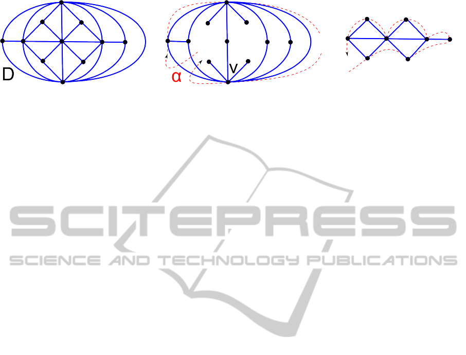
Figure 9: A path α through vertices of the non-hamiltonian maximum planar graph meets any edge at most once.

5 EMBEDDING A GRAPH IN 3

PAGES

The input of our algorithm for drawing an embedding

in 3 pages should be a knotted graph or its plane dia-

gram, which is usually represented on a computer by

a Gauss code. Even for knots an abstract Gauss code

may not represent a closed curve in 3-space. That is

why we ﬁrst solved the planarity problem for Gauss

codes of knotted graphs in Theorem 9.

If we know that a given Gauss code represents a

plane diagram D of a knotted graph G, our next step

in Theorem 11 is to draw the diagram D in a 2-page

book as deﬁned below. After that we upgrade this

topological 2-page embedding of D to a 3-page em-

bedding of G in linear time, see Theorem 12.

Deﬁnition 10. The k-page book consists of k half-

planes with a common boundary line α called the

spine of the book. An embedding of an undirected

graph G into the k-page book is topological if the in-

tersection of G with the spine α is ﬁnite and includes

all vertices of G. A bend of an edge e ⊂ G is any inte-

rior point p of e such that p ∈ α. If every edge of an

embedded graph G is contained in a single page, the

k-page book embedding of G is combinatorial.

A graph D is planar if D can be embedded in R

Any undirected planar graph has a combinatorial 4-

page embedding (Yannakakis, 1989). Figure 9 shows

a planar graph that can not be combinatorially em-

bedded into 2 pages (Bernhart and Kainen, 1979, sec-

tion 5). Any topological 2-page embedding of this

graph will have extra bends where edges intersect the

spine. The linear time algorithm below guarantees at

most one bend per edge for any planar graph.

Theorem 11. (Di Giacomo et al., 2005, Theorem 1)

Given a planar undirected graph D ⊂ R

with |V | ver-

tices, an algorithm of linear time complexity O(|V |)

can draw a topological embedding of the graph D in

the 2-page book with at most one bend per edge.

Two more pictures in Figure 9 illustrate the key

idea how we can construct a non-self-intersecting

path α that passes through each vertex once and inter-

sects each edge at most once. By an isotopic deforma-

tion of R

, the path α can be converted into a straight

spine, which splits the plane into 2 pages. Since all

vertices and crossings of D are in the spine α, we get

a required topological 2-page embedding of D.

We are not going to minimize the number of bends

of edges in a 2-page embedding of a plane diagram

D, because we shall construct 3-page embeddings of

original knotted graphs with a linear number O(|W |)

of total bends in the length of a Gauss code W .

Theorem 12. Given an abstract Gauss code W , an

algorithm of time complexity O(|W |) determines if W

represents a plane diagram of a knotted graph G ⊂ R

and then draws a topological 3-page embedding of a

graph H isotopic to G. Moreover, the graph H has at

most 8|W | intersections with the spine of the book.

Proof. We ﬁrst apply the linear time algorithm from

Theorem 9 to determine if the code W represents a

plane diagram D of a knotted graph G. If yes, we

draw a 2-page embedding of the diagram D ⊂ R

linear time using the algorithm from Theorem 11.

At every crossing in the diagram D, we mark a

short red arc that crosses over another arc in D. The

centers of all these marked arcs are all crossings of D,

which are already in the straight spine α of the 2-page

book. We may slightly deform the embedding of D

by pushing the marked red arcs into the spine α, see

typical cases in the ﬁrst 5 pictures of Figure 10 where

a crossing of D leads to 3 intersections with α.

If the undercrossing arc was in only one page, we

ﬁrst make an additional intersection so that the de-

formed undercrossing arc goes from one page to an-

other and back, see the last 5 pictures of Figure 10

where a crossing leads to 4 intersections with α.

Now we push all marked red arcs into the extra

3rd page attached along α above the diagram D. So

we have upgraded the 2-page embedding of D to a 3-

page embedding of a knotted graph H isotopic to the

original graph G, see Fig. 12, 13.

IVAPP2015-InternationalConferenceonInformationVisualizationTheoryandApplications

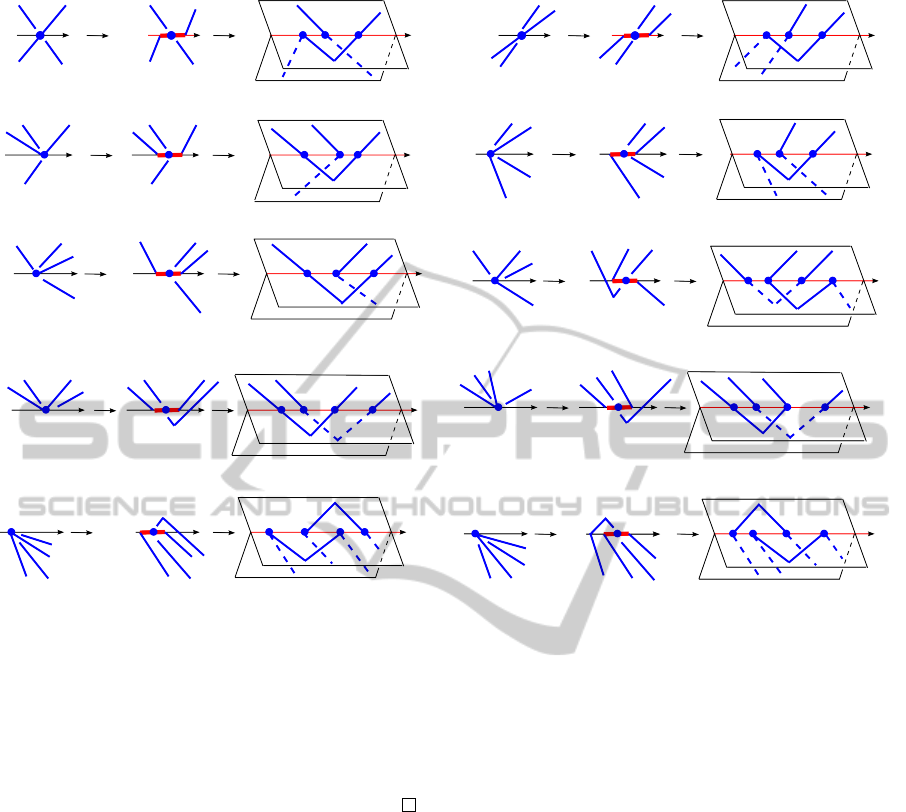
Figure 10: Upgrading crossings to 3-page embeddings.

We need a constant time per crossing, so O(|W |)

in total, for a 3-page embedding of H. Since the

diagram D has |W| edges, the 2-page embedding of

D with at most one bend per edge has at most 2|W |

points in the spine α. Each crossing of D is replaced

by at most 4 intersections with the spine α in a 3-page

embedding of H. The total number of points in the

intersection of H and the spine α is at most 8|W |.

We remind how to encode 3-page embeddings of

all knotted graphs by words in a simple alphabet.

Since edges with vertices of degree 1 can be easily un-

knotted by isotopy in 3-space, for simplicity we con-

sider below only graphs without degree 1 vertices.

To explain the 3-page encoding, let us deform any

3-page embedding so that all arcs are monotonically

projected to the spine α. Then the whole embedding

can be uniquely reconstructed by its thin neighbor-

hood around the spine α. Namely, if we know only

directions of arcs going from points in the spine, we

can uniquely join these arcs in each of 3 pages. Hence

we can encode any 3-page embedding by the list of

local embeddings at all intersections in the spine α.

Theorem 13. (Kurlin, 2007, Theorem 1.6a) Any 3-

page embedding of a knotted graph G with vertices up

to degree n can be encoded by a word in the alphabet

consisting of the letters a

, b

, c

, d

and x

k,i

for each

degree k = 3, . . . , n, where i = 0, 1, 2, see Fig. 11.

Fig. 11 shows 12 local embeddings a

, b

, c

, d

, i ∈

= {0, 1, 2}, that are sufﬁcient for encoding any 3-

page embeddings of knots and links. The notation a

emphasizes that the embeddings a

can be obtained

from each other by a rotation around the spine α.

For encoding graphs in Theorem 13, we can make

sure that at each vertex the spine separates one or

two arcs from others.Then only 3 local embeddings

are enough for each degree, see 3 neighborhoods x

3,0

3,1

, x

3,2

of a degree 3 vertex in Fig. 11.

The 3-page embedding K

⊂ R

in Fig. 3

can be represented by the code w = a

4,1

)

4,1

)(x

4,1

6 DISCUSSION AND PROBLEMS

We now discuss our results in the light of a huge gap

between real-life experiments and pure mathematics.

Experimental data are usually given in the form of un-

structured and noisy clouds of points. If we have only

2D images as in Figure 1, then we also need to extract

a knotted structure in a suitable form.

ALinearTimeAlgorithmforVisualizingKnottedStructuresin3Pages

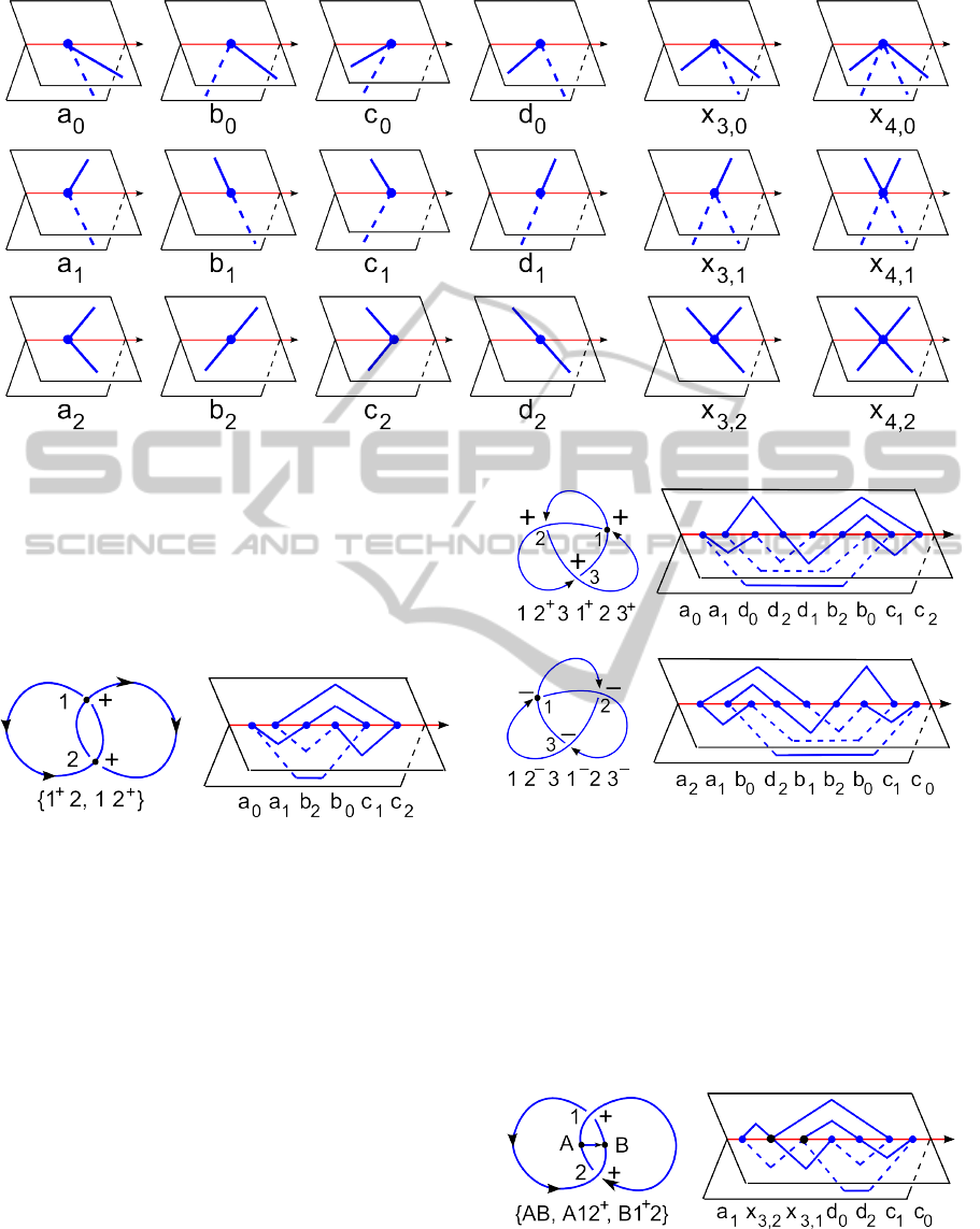
Figure 11: Local 3-page embeddings for the generators of the semigroups from Theorem 14.

Pure mathematicians have developed deep theo-

ries how to classify complicated geometric objects in-

cluding knots. However, all mathematical algorithms

start from ideal models, say a closed curve given by

continuous functions or a polygonal curve given by a

sequence of points connected by straight edges.

Figure 12: Hopf link, its Gauss code, a 3-page embedding.

The key open challenge is to convert any un-

structured experimental data into an ideal theoreti-

cal model that can be rigorously analyzed by exist-

ing mathematical methods. The ﬁrst advance in this

direction is computing the fundamental group of a

knot complement from a point cloud in (Brendel et

al., 2015). We state open problems relating practice

and theory for knotted graphs. We are open to collab-

oration on these problems and related projects.

1. Algorithmically produce a Gauss diagram of a knot

given by a sequence of discrete points in 3-space R

2. Let a link of n components be given as an un-

ordered union of m ≥ 2n open arcs (or sequences of

points). How can we ‘correctly’ join corresponding

endpoints of the arcs to form n closed curves in R

3. When drawing pictures on a tablet, a few intersect-

ing curves can be represented by several sequences

of 2D points sampled along the curves. Under what

Figure 13: Trefoils, Gauss codes, 3-page embeddings.

conditions on the curves and sample, can we quickly

reconstruct the curves using only the sample?

4. Design a fast algorithm to convert an unstructured

3D point cloud sampled around an unknown knotted

structure into a Gauss code W of a knotted graph.

5. Design a robust algorithm to convert a 2D image

of an unknown knotted graph into a Gauss code W .

Figure 14: Hopf graph, its Gauss code, a 3-page embedding.

Our current work on visualizing Gauss codes is

an important step in the hard problems above. First

we may try to recognize small patches of vertices and

IVAPP2015-InternationalConferenceonInformationVisualizationTheoryandApplications

crossings in a 2D image of a knotted graph, but after

that we should combine them in a Gauss codes whose

planarity can be quickly checked by Theorem 9.

Second if we need to visualize any noisy cloud

sampled from an unknown knot K ⊂ R

, we may draw

a knot isotopic to K using its Gauss code and Theo-

rem 12. Even more importantly we often wish to get

a simpliﬁed (minimal) version of a knot.

The state-of-the-art simpliﬁcation algo-

rithm for recognizing trivial knots available at

http://www.javaview.de/services/knots is based on

3-page embeddings. We remind theoretical argu-

ments for extending this 3-page approach to graphs

in Appendix and state more problems below.

6. Design a simpliﬁcation algorithm to untangle dia-

grams of 3D graphs isotopic to planar graphs.

7. Extend our algorithm for drawing graphs in 3 pages

to drawing 2-dimensional surfaces in a universal 3D

polyhedron from (Kearton and Kurlin, 2008).

8. Compute topological invariants of a knotted graph

G ⊂ R

starting from its Gauss code, say the funda-

mental group of the graph complement R

− G.

9. Use the computed invariants to build a database

of isotopy classes of knotted graphs similarly to the

Knot Atlas at http://katlas.math.toronto.edu.

10. Deﬁne a kernel (Sch

olkopf and Smola, 2002)

on point clouds representing knotted graphs so that

one can use tools of machine learning for automatic

recognition of real-life knotted structures in 3D.

Algorithms from Theorems 9 and 12 will be available

on author’s webpage http://kurlin.org. We thank all

reviewers for their helpful suggestions and EPSRC for

funding the author’s secondment at Microsoft.

REFERENCES

Bernhart, F., Kainen, P. (1979) The book thickness of a

graph. J. Combin. Theory B, v. 27, p. 320-331.

Biasotti, S., Giorgi, D., Spagnuolo, Falcidieno, M. (2008)

Reeb graphs for shape analysis and applications. The-

oretical Computer Science, v. 392, p. 5-22.

Brendel, P., Dlotko, P., Ellis, G., Juda, M., Mrozek, M.

(2015) Computing fundamental groups from point

clouds. Applicable Algebra in Engineering, Commu-

nication and Computing, to appear.

Di Giacomo, E., Didimo, W., Liotta, G., Wismath, S. (2005)

Curve-constrained drawings of planar graphs. Com-

putational Geometry, v. 30, p. 1-23.

Enomoto, H., Miyauchi, M. (1999) Lower bounds for the

number of edge-crossings over the spine in a topo-

logical book embedding of a graph. SIAM J. Discrete

Mathematics, v. 12, p. 337-341.

Kauffman, L. (1989) Invariants of graphs in three-space.

Trans. Amer. Math. Soc., v. 311, p. 697-710.

Kearton, C., Kurlin, V. (2008) All 2-dimensional links live

inside a universal 3-dimensional polyhedron. Alge-

braic and Geometric Topology, v. 8 (2008), no. 3, p.

1223-1247.

Kurlin, V. (2007) Dynnikov three-page diagrams of spatial

3-valent graphs. Functional Analysis and Its Applica-

tions, v. 35 (2001), no. 3, p. 230-233.

Kurlin, V. (2007) Three-page encoding and complexity the-

ory for spatial graphs. J. Knot Theory Ramiﬁcations,

v. 16, no. 1, p. 59-102.

Kurlin, V. (2008) Gauss paragraphs of classical links and a

characterization of virtual link groups. Mathematical

Proceedings of Cambridge Phil. Society, v. 145 , no.

1, p. 129–140.

Kurlin, V., Vershinin, V. (2004) Three-page embeddings of

singular knots. Functional Analysis and Its Applica-

tions, v. 38 (2004), no. 1, p. 14-27.

Sch

olkopf, B. and Smola, A. (2002) Learning with kernels.

MIT Press, Cambridge, MA.

Tkalec, U., Ravnik, M., opar, S., umer, S., Muevi, I. (2011)

Reconﬁgurable Knots and Links in Chiral Nematic

Colloids. Science, v. 333, no. 6038 pp. 62–65,

Yannakakis, M. (1989) Embedding planar graphs in four

pages. J. Comp. System Sciences, v. 38, p. 36-67.

APPENDIX

3-page Semigroups

The following result completely reduces the topolog-

ical classiﬁcation of spatial graphs up to isotopy in

3-space to a word problem in some semigroups.

Theorem 14. (Kurlin, 2007, Theorems 1.6 and 1.7)

There is a ﬁnitely presented semigroup whose all cen-

tral elements are in a 1-1 correspondence with all iso-

topy classes of knotted graphs with vertices of degree

up to n. There is a linear time algorithm to determine

if an element belongs to the center of the semigroup.

So two knotted graphs G, H ⊂ R

are isotopic in

3-space if and only if their corresponding central ele-

ments w

, w

are equal in the semigroup. A stronger

result in (Kearton and Kurlin, 2008) says that all iso-

topies between 3-page embeddings are realizable in a

3-dimensional polyhedron (a hexabasic book).

More formally, there are two slightly different

semigroups: RSG

for rigid spatial graphs with ver-

tices up to degree n and NSG

for non-rigid graphs.

Both semigroups have 12 generators a

, b

, c

, d

, i ∈

ALinearTimeAlgorithmforVisualizingKnottedStructuresin3Pages

{0, 1, 2}, and 3(n − 2) generators for vertices up to

degree n, namely 3 generators for each degree from

3 to n, see Fig. 11. The empty word is the unit and

, c

, x

k,i

are not invertible. In the case of links for

n = 2, the semigroup has 48 relations (1)–(4) below,

where i ∈ Z

= {0, 1, 2} is considered modulo 3.

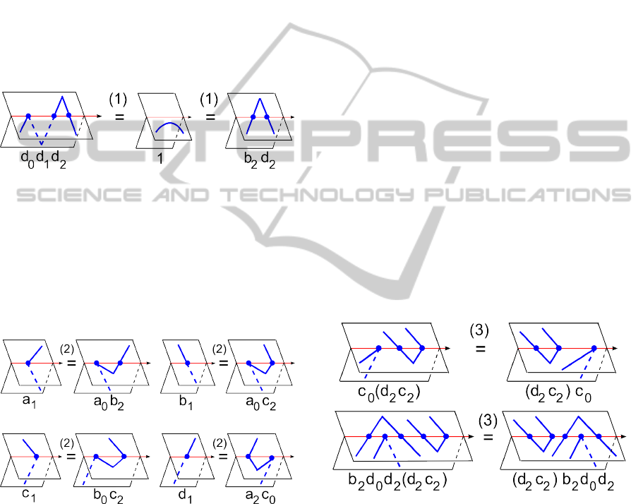
(1) d

= 1 and b

= 1 = d

;

(2) a

= a

i+1

i−1

, b

= a

i−1

i+1

= b

i−1

i+1

, d

= a

i+1

i−1

;

(3) w(d

) = (d

)w for w ∈ { c

i+1

, b

i+1

};

(4) uv = vu, where u ∈ { a

, b

i−1

}

and v ∈ { a

i+1

, b

i+1

, c

i+1

, b

i+1

Figure 15: Relations (1) in the semigroup of Theorem 14.

One of the 7 relations in (1) is superﬂuous as it fol-

lows from the remaining 6. The generators a

, b

, c

, d

can be expressed only in terms of d

, d

, but the result-

ing relations between d

, d

will be longer. All deﬁn-

ing relations of the semigroups represent elementary

isotopies between 3-page embeddings, see typical ex-

amples for relations (1)–(4) in Figures 15–18.

Figure 16: Relations (2) in the semigroup of Theorem 14.

For knotted graphs with vertices of only degree 3,

any non-rigid isotopy can be made rigid, because we

can keep 3 short arcs at any vertex in a moving plane.

Hence both semigroups for rigid and non-rigid iso-

topies from Theorem 14 are the same for n = 3. In

this case the extra relations in addition to (1)-(4) are

(5)–(9), see (Kurlin, 2001) and (Kurlin, 2007):

(5) x

3,i−1

= d

i−1

3,i

i+1

;

(6) x

3,i

i+1

i−1

) = (d

i+1

i−1

3,i

;

(7) x

3,i

= a

3,i

, b

3,i

= a

3,i

;

(8) ux

3,i+1

= x

3,i+1

u for any word u from the set

{ a

, d

, x

3,i

, b

i−1

};

(9) (x

3,i

)v = v(x

3,i

)v for any word v from the set

{ a

i+1

, b

i+1

, c

i+1

, b

i+1

Knotted graphs that have only vertices of de-

gree 4 and are considered up to rigid isotopy are often

called singular knots. Each singular point remains a

transversal intersection of two arcs during a rigid iso-

topy, so the cyclic order of all arcs at any degree 4

vertex is invariant. The semigroup of Theorem 14 for

singular knots has 15 generators a

, b

, c

, d

, x

4,i

, rela-

tions (1)–(4) above and relations (10)–(14) below, see

(Kurlin and Vershinin, 2004) and (Kurlin, 2007):

(10) x

4,i−1

= b

i+1

4,i

i+1

;

(11) (d

4,i

)(d

i+1

i−1

) = (d

i+1

i−1

)(d

4,i

);

(12) d

4,i

= a

4,i

, b

4,i

= a

4,i

;

(13) wx

4,i+1

= x

4,i+1

w for any word w from the set

{ a

, d

4,i

, b

i−1

};

(14) (d

4,i

)v = v(d

4,i

)v for any word v from the

set { a

i+1

, b

i+1

, c

i+1

, b

i+1

The hard part of Theorem 14 says that any isotopy

between graphs decomposes into ﬁnitely many ele-

mentary isotopies involving a small part of a 3-page

code. This is the main advantage of the 3-page en-

coding over plane diagrams and Gauss codes. Indeed,

Reidemeister moves on plane diagrams in Fig. 4 and

their analogues on Gauss codes are not local.

Figure 17: Relations (3) in the semigroup of Theorem 14.

The linear time algorithm for detecting a central

element w checks if the arcs corresponding to all let-

ters of w properly meet each other in every page to

form an embedding of a graph without hanging edges.

For example, the letter a

doesn’t encode any knotted

graph, but a

does, because the arcs of a

and c

meet and form a closed curve in pages 0 and 1.

The 3-page code of a knotted graph commutes

with any other element w in the semigroups from The-

orem 14. For instance, a trivial knot has the code a

and can be isotopically moved in R

to another side

of the 3-page embedding represented by the word w.

IVAPP2015-InternationalConferenceonInformationVisualizationTheoryandApplications

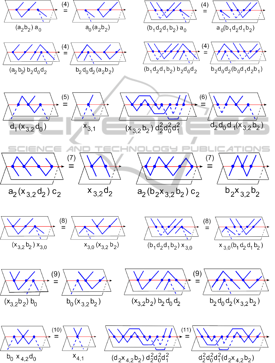
Figure 18: Relations (4) in the semigroup of Theorem 14.

Figure 19: Relations (5)-(6) in the semigroup of Theorem 14.

Figure 20: Relations (7) in the semigroup of Theorem 14.

Figure 21: Relations (8) in the semigroup of Theorem 14.

Figure 22: Relations (9) in the semigroup of Theorem 14.

Figure 23: Relations (10)-(11) in the semigroup of Theorem 14.

ALinearTimeAlgorithmforVisualizingKnottedStructuresin3Pages

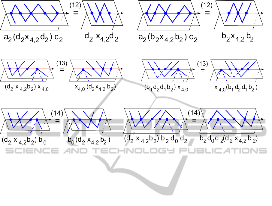
Figure 24: Relations (12) in the semigroup of Theorem 14.

Figure 25: Relations (13) in the semigroup of Theorem 14.

Figure 26: Relations (14) in the semigroup of Theorem 14.

IVAPP2015-InternationalConferenceonInformationVisualizationTheoryandApplications