
A Self-adaptive Likelihood Function for Tracking with Particle Filter
S
´
everine Dubuisson
1
, Myriam Robert-Seidowsky
2
and Jonathan Fabrizio
2
1
CNRS, UMR 7222, ISIR, F-75005, Paris, France
2
LRDE-EPITA, 14-16, rue Voltaire, F-94276, Le Kremlin Bic
ˆ
etre, France
Keywords:
Visual Tracking, Particle Filter, Likelihood Function, Correction Step.
Abstract:
The particle filter is known to be efficient for visual tracking. However, its parameters are empirically fixed,
depending on the target application, the video sequences and the context. In this paper, we introduce a new
algorithm which automatically adjusts online two majors of them: the correction and the propagation param-
eters. Our purpose is to determine, for each frame of a video, the optimal value of the correction parameter
and to adjust the propagation one to improve the tracking performance. On one hand, our experimental results
show that the common settings of particle filter are sub-optimal. On another hand, we prove that our approach
achieves a lower tracking error without needing to tune these parameters. Our adaptive method allows to
track objects in complex conditions (illumination changes, cluttered background, etc.) without adding any
computational cost compared to the common usage with fixed parameters.
1 INTRODUCTION
Visual tracking is an important task in computer vi-
sion with a lot of applications in our daily life, such as
monitoring human-computer interaction for example.
Among all existing trackers, those relying on the par-
ticle filter have become very popular thanks to their
simple algorithmic scheme and efficiency. However,
one of the main drawback of the particle filter is that
it requires to fix two parameters (see Section 2) that
drastically influence the tracking performances. The
first one (σ parameter) is used within the propagation
step, and fixes how far the particles should be diffused
from the current estimated state. The second one (α
parameter) is related to the correction step and influ-
ences how much the likelihood function is peaked.
Although they are essential, they are arbitrarily fixed
in most implementations. In this paper, we propose an
approach that can automatically determine their op-
timal value depending on the temporal context. We
have proven the efficiency of our method on several
challenging video sequences. Moreover, there is no
additional computational cost compared to a version
with fixed parameters.
Only few works discuss the correction parameter
α and the propagation parameter σ settings or their
adaptation over time. The authors in (Fontmarty et al.,
2009) study the impact α and σ values for human
tracking. In their case, they use four specific likeli-
hoods related to the silhouette of the tracked object.
They attempt to tune the α value with respect to an
empirical study on their own data. By observing the
behavior of tracking in different configurations, they
determine its optimal interval of values for each like-
lihood. Although this is a very interesting work, we
can not generalize its conclusion, because the study
was made for a specific context with dedicated like-
lihoods. The work proposed in (Lichtenauer et al.,
2004) is also an empirical study to determine an opti-
mal value for α. Here, different distances for compar-
ing particles and model (gradient direction and Cham-
fer matching) are considered for single and multiple
object tracking cases. Experiments, as for previous
work, permit to determine the optimal range of values
for α. Here again, the choice of the α value highly
depends on the chosen distance. In (Brasnett and
Mihaylova, 2007), a problem of multi-cue tracking
(color, texture and edges) is addressed and an adaptive
scheme for the computation of the correction param-
eter is proposed. To the best of our knowledge, this
is the only work that attempts to provide a general
definition of α value. Authors then propose the fol-
lowing heuristic: α =
1
√
2d
min
. Even if their purpose is
to have a particle set containing as few particles with
low weights as possible, their heuristic is not well jus-
tified. In particular, the adaptation of the α value to
the minimal distance d
min
of the particles set permits
to avoid particles to be located on the tail of the like-
lihood distribution. To our own, this is however im-
446
Dubuisson S., Robert-Seidowsky M. and Fabrizio J..
A Self-adaptive Likelihood Function for Tracking with Particle Filter.
DOI: 10.5220/0005260004460453
In Proceedings of the 10th International Conference on Computer Vision Theory and Applications (VISAPP-2015), pages 446-453
ISBN: 978-989-758-091-8
Copyright
c
2015 SCITEPRESS (Science and Technology Publications, Lda.)

portant for some particles to have high weights, but
also for some of them to have low weights to pre-
serve a diversity within the particle set. Note that a
similar work was proposed in (Ng and Delp, 2009).
Except for the latter article, previous solutions rely on
empiric tests and thus, are dedicated to specific track-
ing contexts. In this paper, we propose an algorithm
that can adapt α and σ values over time depending
on the context. It uses a single and simple criterion
based on a potential survival rate and the maximum
weight of the particles set. The paper is organized as
follows. Section 2 presents the particle filter and its
current implementation. It also explains the role of
the propagation and correction parameters. Section 3
details our approach to online automatically adapt α
value and correct σ if necessary. Section 4 gives ex-
perimental results via both qualitative and quantitative
evaluations. Finally, concluding remarks are given in
Section 5.
2 PARTICLE FILTER
Theoretical Framework. The goal of particle fil-
ter’s framework (Gordon et al., 1993) is to estimate a
state sequence {x
t
}
t=1,...,T
, whose evolution is given
from a set of observations {y
t
}
t=1,...,T
. From a proba-
bilistic point of view, it amounts to estimate for any t,
p(x
t
|y
1:t
). This can be computed by iteratively using
Eq. (1) and (2), which are respectively referred to as
a prediction step and a correction step.
p(x
t
|y
1:t−1
) =
R
x
t−1
p(x
t
|x
t−1
)p(x
t−1
|y
1:t−1
)dx
t−1
(1)
p(x
t
|y
1:t
) ∝ p(y
t
|x
t
)p(x
t
|y
1:t−1
) (2)
In this case, p(x
t
|x
t−1
) is the transition and
p(y
t
|x
t
) the likelihood. Particle filter aims at approx-
imating the above distributions using weighted sam-
ples {x
(i)
t
,w
(i)
t
} of N possible realizations of the state
x
(i)
t
called particles.
The global algorithm of particle filter between
times steps t −1 and t is summarized below.
1. Represent filtering density at t −1 p(x
t−1
|y
1:t−1
)
by a set of weighted particles (i.e. samples)
{x
(i)
t−1
,w
(i)
t−1
}, i = 1, . . . , N
2. Explore the state space by propagating sam-
ples using a proposal function so that x
(i)
t
∼
q(x
t
|x
0:t−1
,y
1:t
).
3. Correct samples by computing particle’s weight
so that:
w
(i)
t
∝ w
(i)
t−1
p(y
t
|x
(i)
t
)p(x
(i)
t
|x
(i)
t−1
)
q(x
(i)
t
|x
(i)
0:t−1
,y
1:t
)
(3)
with
∑
N
i=1
w
(i)
t
= 1
4. Estimate the posterior density at t by the weighted
samples {x
(i)
t
,w
(i)
t
}, i = 1, . . . , N, i.e.
p(x
t
|y
1:t
) ≈
N
∑
i=1
w
(i)
t
δ
x
(i)
t
(x
t
)
where δ
x
(i)
t
are Dirac masses centered on particles.
5. Resample (if necessary)
Model for Implementation. Two densities are fun-
damental for particle filter: the propagation and the
likelihood ones.
The first one permits to get the prior of
the estimation, and rely on the proposal density
q(x
t
|x
0:t−1
,y
1:t
). The most common choice for this
proposal is the transition density p(x
t
|x
t−1
). The re-
sulting recursive filter is also called Bootstrap filter,
or CONDENSATION (Gordon et al., 1993). Be-
cause the motion of the tracked object is unknown,
the transition function is often modeled by a Gaus-
sian random walk centered around the current estima-
tion x
t−1
. We then get p(x
t
|x
t−1
) ∼G(x
t−1
,Σ), where
G is a Gaussian with mean x
t−1
and covariance ma-
trix Σ. The variances σ (in the diagonal of Σ) fix how
far the particles are propagated from x
t−1
. The higher
these variances, the further particles are propagated.
When using transition function as proposal, Eq. 3
becomes w
(i)
t
∝ w
(i)
t−1
p(y
t
|x
(i)
t
). In such a case, parti-
cles’ weights are proportional to the likelihood, and
if we only consider the current observation, we get
w
(i)
t
∝ p(y
t
|x
(i)
t
). According to the common model-
ing of the likelihood, the second fundamental den-
sity is p(y
t
|x
(i)
t
) ∝ e
−αd
2
, where e is the exponential
function, d is a similarity measure (d ∈ [0,1]) that
indicates the proximity between particle x
(i)
t
and the
model of the tracked object. Usually, the tracked ob-
ject is modeled by the histogram of its surrounding
region, and d is the Bhattacharya distance (Bhat-
tacharyya, 1943). Parameter α influences how peaked
is the likelihood function: if α value is high (resp.
small), then the likelihood will be peaked (resp.
spread out).
Influence of Parameters. As we previously stated,
two parameters are very important and hard to fix.
Table 1 shows for example, how tracking errors can
drastically increase depending on the choice of α
value. We describe below their role.
The propagation parameter (σ) corresponds to the
variance that defines how far from the current estima-
tion the particles are propagated. If its value is too
high (resp. too small), then particles are propagated
ASelf-adaptiveLikelihoodFunctionforTrackingwithParticleFilter
447

too far (resp. too close). Thus, the tracking will prob-
ably fail because only a small number of particles are
well located in the state space.
The correction parameter (α) allows to adjust the
spread of the likelihood. This is illustrated in Fig. 1,
where the target is the person on the middle bottom of
frames (surrounded by a red box). We show the like-
lihood maps (Bhattacharyya distance between color
histograms, see Section 4) for different values of α. A
white pixel (resp. black) correspond to a high (resp.
low) likelihood value. As can be seen, when α value
is small (α = 1), large areas of the map have high
values. Therefore, many particles get a high weight,
even those far from the real object position. With such
a small value for α the global estimation (weighted
sum of particles) will probably be incorrect. For the
case of α = 100, the white areas are very small: only
a small subset of particles will get high weight. If no
particle were previously propagated onto this small
high likelihood area, then the global estimation will
also be incorrect.
Figure 1: Influence of the α parameter of the likelihood
function. From left to right: the original image (the model
is the histogram of the region surrounding the person on
middle bottom), likelihoods maps with α = 1 and α = 100.
In the literature (Hassan et al., 2012; Maggio et al.,
2007; Erdem et al., 2012; P
´
erez et al., 2002) these
parameters are empirically fixed, depending on the
tested sequences or the target application. Then, α
is tuned to fix the spread of the likelihood so that its
high value areas approximately cover the region sur-
rounding the tracked object. Variances σ
w
and σ
h
are
also fixed depending on the motion in the sequence:
large values for high motion, and small ones for low
motion. Moreover, these two parameters are defined
for all the sequence: if the motion or appearance of
the tracked object changes, as well as its surrounding
context, the tracking will probably fail because these
parameters are not well adapted anymore. In this pa-
per, we propose an algorithm to adapt the propaga-
tion and correction parameters to each frame of the
sequence without any additional cost in term of com-
putation time. This is done by analyzing the disper-
sion of the particle set in order to determine if it is
still adapted to the current context. If it is not adapted
anymore, the parameters are changed to make this set
suitable. Our approach is described in the next sec-
tion.
3 PROPOSED APPROACH
In the particle filter framework, a resampling step can
be necessary (step 5 of algorithm given in Section 2)
in cases of degeneration of the particle set, i.e. when
most of the particles have a low weight. It means
the variance of the particle set is too high. Usually,
the particle set is resampled when its associated ef-
ficient number becomes higher than a given thresh-
old (Gordon et al., 1993). This number is computed
from the normalized weights and monitors the amount
of particles that significantly contribute to the poste-
rior density. It is given by N
e f f
t
=
1
∑
N
i=1
w
(i)
t
2
. Note
that, this number does not permit to distinguish a bad
particle set (only low weights) from a very good par-
ticle set (only high weights). Indeed, for both cases,
after the weight normalization, all particles get simi-
lar weights (around 1/N), and the efficient number a
similar value. This shows the difficulty to fix a gen-
eral threshold on this efficient number to determine
whether or not the particle set is correct and does not
need to be resampled. However, it provides a good in-
dication on the number of particles with high and low
weights. As previously said, intuitively, we would
like that most particles have high weights, but some
also get low weights, to preserve the diversity of the
particle set. For example, if a proportion of 0.5 of the
particle set have high weights (around 2/N after nor-
malization), the remainder with low weights (around
0 after normalization), then N
e f f
t
≈
N
2
. Then, if a pro-
portion of p particles have high weights, N
e f f
t
≈ N p.
Here we call p the survival rate.
In this paper, we adopt an opposite reasoning than
usually. Instead of adapting the particle set to the like-
lihood by resampling the former, we adapt the likeli-
hood to the particle set. We search for the α value that
provides a specific efficient number. Our idea is to de-
termine which α value permits to reach this equality:
N
e f f
t
≈ max
i
(w
(i)
t
). This corresponds to a proportion
p ≈
max
i
(w
(i)
t
)
N
of particles with high weights. Fig. 2
shows two plots of the survival rate p (in red) and
the maximum weight (in green) depending on the α
value. As can be seen, the efficient number decreases
when α increases because the number of particles
with high weight usually decreases in cases of peaked
likelihoods. On the contrary, the maximum weight
value increases with α because high likelihood values
are distributed in smaller areas. These curves have an
intersection point, whose abscissa gives our optimal α
value. The choice of max
i
(w
(i)
t
) also permits to detect
if the particle set was not well propagated, i.e. if σ
does not suit the target’s motion. If there is no inter-
VISAPP2015-InternationalConferenceonComputerVisionTheoryandApplications
448

section between p and max
i
(w
(i)
t
) curves, it means, ei-
ther the maximum weight has a very high value (close
to an impoverishment problem), or a low one (close
to the degeneracy issue). In this case, we increase σ
value and re propagate particle set, and then search
again for the optimal α. Our algorithm is summarized
in Algorithm 1. Here BD(.,.) is the Bhattacharyya
distance between the model and particle descriptors.
0 50 100 150 200 250 300 350 400 450 500
0
0.1
0.2
0.3
0.4
0.5
0.6
0.7
0.8
0.9
1
Alpha value
Efficient number
Maximum weight
0 50 100 150 200 250 300 350 400 450 500
0.1
0.2
0.3
0.4
0.5
0.6
0.7
0.8
Alpha value
Efficient number
Maximum weight
Figure 2: Plots of survival rate and maximum weight values
depending on α value for a particle set (N = 20), between
frames 1 and 2 of sequences Crossing and Liquor.
Input: Image I
t
, particle set {x
(i)
t−1
,w
(i)
t−1
}
N
i=1
Particle set {x
(i)
t
,w
(i)
t
}
N
i=1
, α
init
, σ
init
α
max
, α
update
, σ
max
Output: Optimal α value α
opt
1 di f f ← 1, α ←α
init
, σ ←σ
init
2 x
(i)
t
∼ G(x
(i)
t−1
,σ)
3 D
(i)
t
← BD
2
(.,.), i = 1, ... ,N
4 while di f f > 0 and α ≤α
max
and σ ≤σ
max
do
5 w
(i)
t
← e
−αD
(i)
t
, i = 1,. .., N
6 p =
1
N
∑
N
i=1
w
(i)
t
2
7 di f f = p −max
i
(w
(i)
t
)
8 if α = α
max
then
9 σ ←2σ
10 x
(i)
t
∼ G(x
(i)
t−1
,σ)
11 D
(i)
t
← BD(.,.), i = 1, ... ,N
12 α ←α
init
13 α ←α + α
update
14 α
opt
← α −α
update
Algorithm 1: Algorithm for the selection of optimal α for
correction and σ adaptation for propagation.
4 EXPERIMENTAL RESULTS
In this section, we show the efficiency of our proposed
algorithm to increase tracking accuracy. We first give
our experimental setup in Section 4.1. Quantitative
results are then given in Section 4.2. Finally, 4.3 pro-
pose a study of the interest of our approach in com-
plex tracking situations and its convergence, stability
and computations times.
4.1 Experimental Setup
In this paper, we use the same experimental setup for
all tests provided. This setup is given below.
The state vector contains the parameters describ-
ing the object to track, and is defined by x
t
= {x
t
,y
t
},
with {x
t
,y
t
} the central position in the current frame
of the tracked object. A particle x
(i)
t
= {x
(i)
t
,y
(i)
t
},
i = 1, . . . , N, is then a possible spatial position of this
object.
The observation model is computed into a fixed
size region surrounding the state position. This model
is manually initialized in the first frame of the se-
quence (from the ground truth associated with the
tested sequences - see Section 4.2). We have tested
two different descriptors for surrounding regions. The
first one, called M
col
, is the color histogram. It is
build by concatenating the 8-bin histograms of the
three RGB channels to get a 24-bin histogram. The
second one, M
col+hog
contains both color and shape
information. The color information is the same as
in M
col
. The shape information is the concatenation
of two 8-bin histograms of gradient (HOG) (Dalal
and Triggs, 2005) computed in the upper and bot-
tom parts of the region. Then, we get two histograms
for M
col+hog
: a 24-bin color histogram plus a 16-bin
HOG. These descriptors will be used for the observa-
tion model and each particle’s region.
Particles are propagated using a Gaussian random
walk whose variance is fixed depending on the size
of the region surrounding the tracked object. Know-
ing h and w respectively the height and width of this
region (fixed and given by the ground truth), we use
σ
w
= w/2 and σ
h
= h/2 as propagation parameters
(note that in our algorithm, σ is adapted over time if
necessary).
Particles’ weights are computed in two different
ways, depending on the descriptor. For M
col
de-
scriptor, we compute w
(i)
t
∝ e
−αd
2
col
, where d
col
is the
Bhattacharyya distance between the color histogram
of the model and the one of the target. For de-
scriptor M
col+hog
, we compute w
(i)
t
∝ e
−α(d
col
×d
hog
)
2
,
where d
hog
is the Bhattacharyya distance between the
model’s HOG and particle’s one.
The current estimation of the tracked objects’ po-
sition is the weighted sum of particles positions.
A multinomial resampling (Gordon et al., 1993) is
done at the end of each time step.
For all tests, we fixed N = 20. Algorithm 1 also
requires to fix some parameters concerning the initial-
ization, update and maximum value of α. We always
use the same parameters: α
init
= 10, α
update
= 10,
α
max
= 500, σ
max
= 10. M
re f
is the descriptor of the
ASelf-adaptiveLikelihoodFunctionforTrackingwithParticleFilter
449

model i.e. object to track and M
(i)
t
is the one of the
i
th
particle in the frame t. diff is the criterion to deter-
minate the intersection between the two curves.
4.2 Quantitative Results
In order to evaluate our approach, we use the Tracker
Benchmark from (Wu et al., 2013). It contains 50
challenging sequences with various visual tracking
difficulties (illumination changes, deformation, rota-
tion, scale changes of the target and the context, etc.).
All sequences are provided with their ground truth,
that permits to perform a quantitative evaluation.
We compare tracking errors obtained with our ap-
proach, with a classical approach that uses fixed val-
ues used for α (20, 50, 100 and 200). We also com-
pare our method with the one in (Brasnett and Mi-
haylova, 2007), i.e. α =
1
√
2d
min
. We tested the two
descriptors M
col
and M
col+hog
. Table 1 gives tracking
errors obtained by all methods on some sequences of
the benchmark (all sequences have been tested), cor-
responding to a mean over 10 runs. This table shows
our approach gives most of times lower tracking er-
rors (in bold) for both models. Overall the sequences,
our tracking errors, compared to other approaches,
are from 13% to 20% lower with descriptor M
col
and
from 24% to 33% lower with descriptor M
col+hog
.
We can also highlight that for fixed α, lower track-
ing errors are never get with the same α value (see
underlined scores), showing there is no universal α
value. The approach suggested in (Brasnett and Mi-
haylova, 2007) sometimes gives lower tracking errors
than with all fixed α, but often a specific fixed α value
achieves better results. However, it does not achieve
as lower errors as our approach does, except for two
cases (Trellis and Skiing sequences).
Furthermore, we note some cases where our ap-
proach does not give the lowest tracking errors and
they can be classified into two main classes. First,
cases where our tracking errors are not the best but
very close to the lower tracking error (see for exam-
ple sequences Mhyang or Freeman1). Secondly, cases
of divergence of the particle filter: for all approaches
including ours, tracking errors are very high. Indeed,
the benchmark contains very complicated sequences,
such like Ironman for example (moving camera, high
deformations, strong motions, occlusions, etc.).
Moreover, we have compared the tracking er-
rors obtained with our method and errors obtained
for fixed α values ranging from 10 to 500 (step of
10). Results are given in Fig. 3 for two sequences
(Football1, and Matrix). Each plot are tracking er-
ror (mean over 10 runs) obtained with different fixed
value for α (blue curves). One can see errors ob-
tained with our approach (red lines) are always lower
than the lower error given using a specific and fixed
α value. These plots show how much the errors with
fixed α are not stable. This, once again, demonstrates
the impact of the α value and the difficulty of choos-
ing a good one adapted for a whole sequence and even
more generally to a set of sequences.
0 50 100 150 200 250 300 350 400 450 500
10
20
30
40
50
60
70
80
90
100
110
Alpha value
Error (in pixels)
0 50 100 150 200 250 300 350 400 450 500
75
80
85
90
95
100
105
110
115
120
Alpha value
Error (in pixels)
Figure 3: Variation of tracking errors (N = 20), depending
on the value of α (fixed for all the frame). In red: track-
ing error obtained with our approach. From top to bottom,
sequences Football1 and Matrix.
All these results point out that the online modifica-
tion over the time of the α value allows our algorithm
to decrease tracking errors. In the next section, we
will show how our self-adaptive likelihood function
performs in specific tracking context.
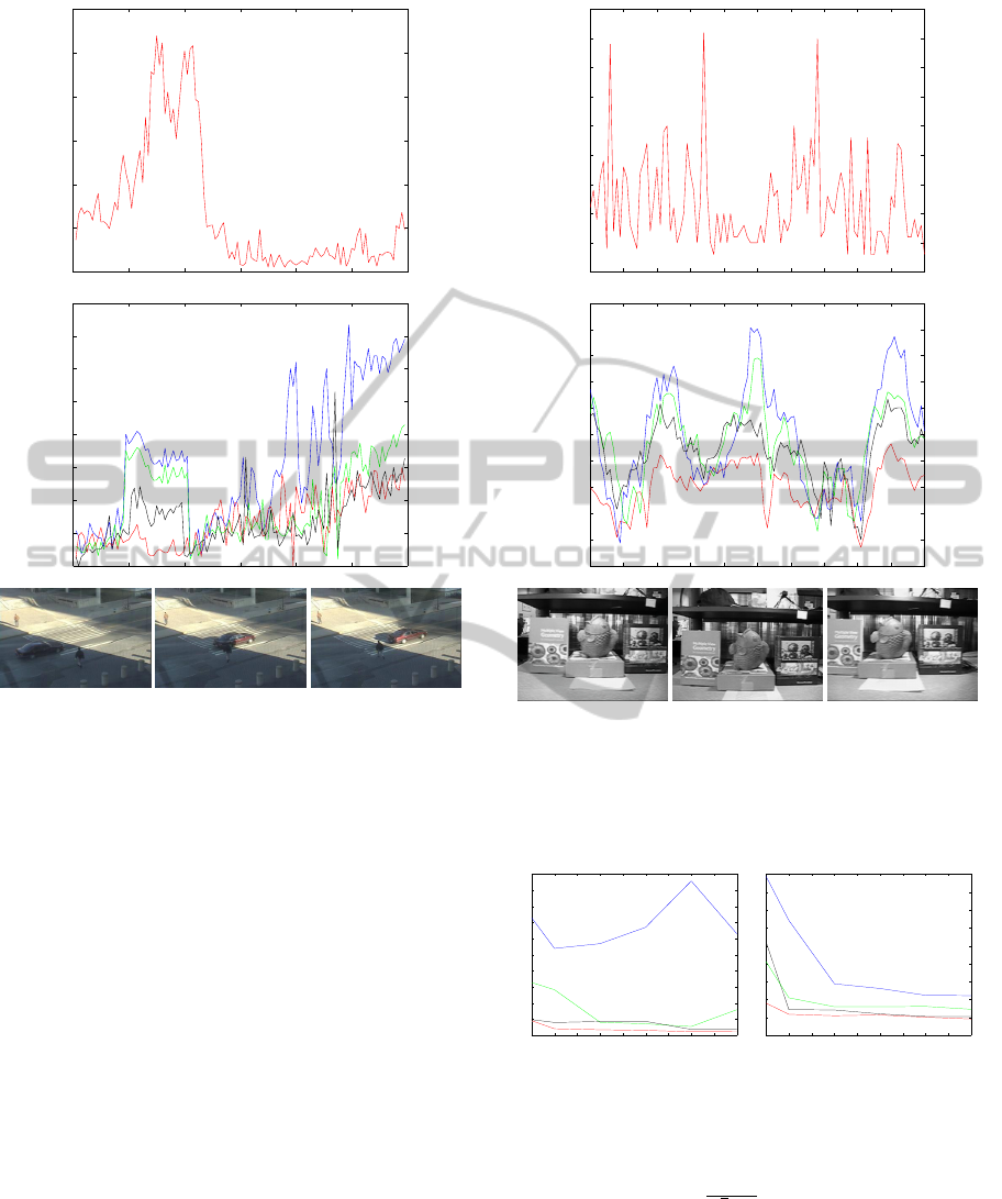
4.3 Complex Tracking Conditions
Proximity between Similar Color Objects. Fig-
ure 4 gives the best α values selected at each frame by
our algorithm for the Crossing sequence, in which
we attempt to track the person on the bottom (using
M
col
). As can be seen on this figure, during frame
interval [20,50], α gets high values, while after and
before this interval time it gets low values. Indeed, in
this sequence, during this interval of time, a car gets
very close to the tracked person (see on the bottom of
this figure, frames 20, 40 and 50). As its color is simi-
lar, a large region of the likelihood around the tracked
people gets high values. Usually, the tracking with a
fixed value for α would be disturbed, because a lot of
VISAPP2015-InternationalConferenceonComputerVisionTheoryandApplications
450

Table 1: Tracking errors obtained on some sequences among the 50 of Tracker Benchmark proposed in (Wu et al., 2013) for
different approaches. Lower tracking errors are in bold and lower given by a fixed α are underlined.
M
col
: Color histogram M
col+hog
: HOG + Color histogram
Our α = α = α = α = α = Our α = α = α = α = α =
Sequence α adapt.
1
√
2d
min
20 50 100 200 α adapt.
1
√
2d
min
20 50 100 200
Sylvester 18.1 23.6 19.0 19.1 18.1 18.5 8.2 28.8 10.4 8.9 9.1 8.2
Trellis 71.6 64.1 71.9 78.2 78.0 80.6 66.0 72.3 119.5 70.4 78.5 78.9
Fish 34.5 52.3 37.5 34.8 34.5 35.3 23.7 41.5 30.8 27.9 24.6 25.1
Mhyang 16.5 32.1 16.9 16.3 16.4 16.7 14.6 23,7 15.4 14.8 29.3 29.0
Matrix 76.1 79,1 105.7 87.6 95.7 91.9 64.4 71.2 82.2 90.2 100.2 78.3
Ironman 118.9 148.4 135.3 147.4 158.6 159.0 114.3 154.8 143.3 178.2 113.0 200.6
Deer 46.0 92.9 75.7 86.2 50.3 57.8 59.1 81.6 77.8 112.6 210.4 59.7
Skating1 68.0 91.3 103.7 85.8 91.1 89.5 44.2 66.2 81.9 51.3 57.2 83.5
Boy 32.8 72.3 39.5 48.2 63.4 60.6 14.1 53.7 44.0 33.3 33.5 34.8
Dudek 71.8 161.4 110.3 80.5 84.3 85.4 44.2 101.2 91.9 161.4 48.4 58.0
Crossing 7.7 86.7 23.3 8.8 8.6 8.5 5.1 29.3 7.6 5.8 5.4 5.6
Couple 15.6 28.8 35.3 17.9 17.3 17.2 14.2 19.5 20.1 62.1 16.8 18.2
Football1 12.5 53.9 25.8 17.7 14.9 15.4 11.7 28.2 20.7 18.2 13.6 13.1
Freeman1 43.5 99 46.8 62.1 42.9 56.3 15.0 18.4 16.4 15.6 15.3 19.2
Jumping 42.9 53.5 50.8 46.4 44.4 50.9 54.7 68.5 100.7 60.2 57.7 56.0
CarScale 47.4 47.5 59.6 60.9 48.2 54.1 33.6 51.2 62.1 59.1 60.4 45.2
Skiing 238.9 178.0 237.3 263.0 266.9 276.2 211.2 166.1 196.1 227.0 264.9 225.8
Dog1 17.1 24.8 21.4 18.9 17.5 17.6 47.4 48.0 50.0 50.0 50.4 49.5
MoutainBike 22.2 84.6 28.8 40.0 30.9 35.6 11.3 96.0 20.3 18.0 11.9 17.5
Lemming 43.6 127.0 122.3 81.5 91.9 78.2 101.8 125.2 209.6 138.2 119.3 244.2
Liquor 46.4 53.1 69.1 59.2 54.3 57.1 38.2 45.9 67.5 52.3 43.3 42.4
Faceocc2 48.1 57.9 51.4 63.0 54.6 55.1 35.8 49.2 41.7 59.4 58.9 41.0
Basketball 83.1 85.6 86.5 87.1 85.8 83.7 40.4 62.2 184.5 99.3 82.4 54.6
Football 118.5 122.6 178.0 170.6 203.8 210.5 109.6 118.2 185.9 219.5 227.1 234.0
Mean (over 50 seq.) 62.3 78.7 78.7 75.2 74.5 71.8 49.6 64.4 74.4 69.6 65.2 66.4
particles will get high weights, even those far from the
tracked person, or on the other object with a similar
color. To better track the person, it is then necessary
for the likelihood to be more peaked on the tracked
object, that is the reason why α should get high val-
ues during this time. We see on this example that our
approach is able to adapt to the context (i.e. two ob-
jects with similar colors close to each other).
Middle plot of this figure corresponds to track-
ing error curves obtained with our algorithm (red
curve), and fixed values over all the sequence, α =
20 (blue curve), α = 50 (green curve) and α = 100
(black curve). Thanks to our automatic selection of
α value, our tracking errors decrease during interval
time [20, 50], contrary with those obtained with fixed
α. Globally, on Crossing sequence, our approach
provides an average error of 7.7%, while errors with
α = 20, α = 50 and α = 100 are respectively 23.3%,
8.8% and 8.6%.
Illumination Changes. At the end of the Crossing
sequence (from approximately frame 80), there is an
illumination change. However, our approach is less
disturbed: its errors are the lowest, while they can
drastically increase with a bad fixed value for α (see
for α = 20 for example). Fish sequence shows a toy
slowly moving under a light (see some frames on the
bottom of Fig. 5). The illumination conditions are
hardly changing, and the color model, fixed over time,
is not adapted to efficiently track the object during the
sequence. Fig. 5 presents the evolution of optimal α
values over time, during frames [200 −300]. As can
be seen, its value often change with time, due to the
changes in illumination. Tracking errors are shown in
the middle plot of this figure: our method (red curve)
is more stable with time than the others. This illus-
trates the interest of our approach to better track with
time in such conditions.
These tests have proven that our automatic adapta-
tion of the α value allows to improve tracking perfor-
mances (i) in case of proximity between similar color
objects and (ii) in case of illumination changes. In-
deed, in such cases, most of times the modes of the
likelihood can become very spread out or peaked: in-
creasing or decreasing α value permits to adapt our
correction step to the current context.
Convergence Study. All our previous tests were
made with N = 20 particles, this is important to check
if our approach does not get the best results only with
a small number of particles. We then give in Fig. 6
convergence curves, i.e. errors depending on the num-
ASelf-adaptiveLikelihoodFunctionforTrackingwithParticleFilter
451
0 20 40 60 80 100 120
50
100
150
200
250
300
350
Frame number
Alpha optimal
0 20 40 60 80 100 120
0
10
20
30
40
50
60
70
80
Error (in pixels)
Frame number
Figure 4: Crossing sequence. Top: optimal α selected by
our approach along the sequence (120 frames, mean over
30 runs). Middle: tracking errors obtained with our ap-
proach (red) and with fixed α = 20 (blue), α = 50 (green)
and α = 100 (black). Bottom: frames 20, 40 and 50, i.e. be-
fore, during and after the car and the walking tracked person
trajectories cross.
ber of particles for two video sequences (Walking and
Couple). In these plots, we compare results obtained
with fixed α (20, 50 and 100) values and our adaptive
α. We can see our approach always converges faster
and better. This proves we could use less particles to
achieve lower tracking errors than with fixed α.
Stability. We previously explained that our ap-
proach which adapts the correction step permits a bet-
ter and faster convergence of the tracker compared to
approaches with a fixed α value. We reported in Ta-
ble 2 some comparisons of variances obtained over
10 runs with descriptor M
col
. As can be seen, our al-
gorithm also reduces the variance over the runs, that
proves its stability. Indeed, the variance over the runs
is highly dependent on the random generation of sam-
ples (propagation): if the set of particles is badly
propagated, a particle filter with a fixed α will proba-
bly fail in correctly tracking. On the contrary, our ap-
proach permits α to adapt the likelihood to the prop-
200 210 220 230 240 250 260 270 280 290 300
50
100
150
200
250
300
350
400
450
500
Frame number
Alpha value
200 210 220 230 240 250 260 270 280 290 300
15
20
25
30
35
40
45
50
55
60
65
Frame number
Error (in pixels)
Figure 5: Fish sequence (frames 200 to 300). Top: optimal
α selected by our approach along the sequence (100 frames
out of 476, mean over 30 runs). Middle: tracking errors ob-
tained with our approach (red) and with fixed α = 20 (blue),
α = 50 (green) and α = 100 (black). Bottom: frames 205,
240 and 290, i.e. when object is lighted or not.
10 20 30 40 50 60 70 80 90 100
20
40
60
80
100
120
140
160
180
200
220
Number of particles
Error (in pixels)
10 20 30 40 50 60 70 80 90 100
10
15
20
25
30
35
40
45
50
55
Error (in pixels)
Number of particles
Figure 6: Convergence curves according to the number par-
ticles for Walking and Couple sequences. In red our ap-
proach, in blue α = 20, in green α = 50, in black α = 100.
agated particle set, that makes it more stable. Note
that when using α =
1
√
2d
min
heuristic, we get similar
or lower variances than with fixed α, but not as small
as our variances.
About Computation Times. Our tests show that
our approach does not add an additional computa-
tional cost. Indeed, computation times are similar
whether we use a fixed α or adapt it over time. In par-
VISAPP2015-InternationalConferenceonComputerVisionTheoryandApplications
452

Table 2: Stability (variance of tracking errors over 10 runs)
obtained with fixed and adaptive α on several video se-
quences. The lowest in bold.
Our α = α = α = α = α =
Sequence α adapt.
1
√
2d
min
20 50 100 200
CarDark 0.4 12.8 23.5 20.0 22.7 18.9
Fish 0.2 0.6 0.7 0.3 0.4 0.4
Matrix 7.9 14.6 15.3 12.7 18.8 9.5
Couple 1.2 3.1 2.5 1.5 2.4 2.0
CarScale 4.3 7.1 6.3 5.6 5.1 7.2
Football 2.2 29.8 93.5 41.1 34.8 43.9
Dog1 2.3 5.1 3.9 4.2 3.9 10.2
ticle filter, the most time consuming step is the correc-
tion one, more precisely the computation of distances
between particles and model. This step is done once,
for fixed or adaptive α. Our algorithm is just a loop
over all possible values for α (form 10 to 500, with
a step of 10), that corresponds to a maximum of 50
values. This is why our optimal α does not add any
cost to the global particle filter algorithm. Note that
sometimes our computation times are lower: because
our likelihood density is better adapted to the particle
set, the resampling can require less time. We get an
average of +0.42% of the computation times for all
50 tested sequences.
5 CONCLUSION
In this paper, we have presented an approach that au-
tomatically adapts over time fundamental parameters
of the likelihood function of the particle filter. More
precisely, using a single and simple criterion, it can
set the correction parameter as well as the propaga-
tion parameter. Moreover, it does not require any ad-
ditional cost in term of computation times.
Our tests have proven on several and challenging
video sequences the high impact of these two param-
eters on the tracking performances. However, they
are often neglected and set up with fixed and arbi-
trary values that can, as we have shown, increase the
tracking errors. Our experiments also show, that our
method which adapts these parameters depending on
the context greatly improves the robustness of the par-
ticle filter. Moreover, it converges better, faster and
is more stable. Particularly, our algorithm still suc-
ceeds in complex tracking situations like illumination
changes or proximity between similar color objects.
Further works will concern the validation of our
approach by using different kinds of descriptors (such
as wavelets), similarity measures (such as Chamfer)
in order to prove the generalization of our technique.
We also attempt to show our approach can also im-
prove multi-cue or multi-modal tracking accuracies.
Finally, we are working on the derivation of a mathe-
matical demonstration of the validity of our criterion
used to determine the optimal correction value.
REFERENCES
Bhattacharyya, A. (1943). On a measure of divergence
between two statistical populations defined by their
probability distributions. Bulletin of Cal. Math. Soc.,
35(1):99–109.
Brasnett, P. and Mihaylova, L. (2007). Sequential monte
carlo tracking by fusing multiple cues in video se-
quences. Image and Vision Computing, 25(8):1217–
1227.
Dalal, N. and Triggs, B. (2005). Histograms of oriented
gradients for human detection. In CVPR, pages 886–
893.
Erdem, E., Dubuisson, S., and Bloch, I. (2012).
Visual tracking by fusing multiple cues with
context-sensitive reliabilities. Pattern Recognition,
45(5):1948–1959.
Fontmarty, M., Lerasle, F., and Danes, P. (2009). Likelihood
tuning for particle filter in visual tracking. In ICIP,
pages 4101–4104.
Gordon, N., Salmond, D., and Smith, A. (1993). Novel ap-
proach to nonlinear/non-Gaussian Bayesian state esti-
mation. IEE Proc. of Radar and Signal Processing,
140(2):107–113.
Hassan, W., Bangalore, N., Birch, P., Young, R., and
Chatwin, C. (2012). An adaptive sample count parti-
cle filter. Computer Vision and Image Understanding,
116(12):1208–1222.
Lichtenauer, J., Reinders, M., and Hendriks, E. (2004). In-
fluence of the observation likelihood function on ob-
ject tracking performance in particle filtering. In FG,
pages 767–772.
Maggio, E., Smerladi, F., and Cavallaro, A. (2007). Adap-
tive Multifeature Tracking in a Particle Filtering
Framework. IEEE Transactions on Circuits and Sys-
tems for Video Technology, 17(10):1348–1359.
Ng, K. K. and Delp, E. J. (2009). New models for real-
time tracking using particle filtering. In VCIP, volume
7257.
P
´
erez, P., Hue, C., Vermaak, J., and Gangnet, M. (2002).
Color-Based Probabilistic Tracking. In ECCV, pages
661–675.
Wu, Y., Lim, J., and Yang, M.-H. (2013). Online object
tracking: A benchmark. In CVPR, pages 2411–2418.
ASelf-adaptiveLikelihoodFunctionforTrackingwithParticleFilter
453
