
Faster Approximations of Shortest Geodesic Paths on Polyhedra
Through Adaptive Priority Queue
William Robson Schwartz
1
, Pedro Jussieu de Rezende
2
and Helio Pedrini
2
1
Department of Computer Science, Universidade Federal de Minas Gerais, Belo Horizonte-MG 31270-010, Brazil
2
Institute of Computing, University of Campinas, Campinas-SP 13083-852, Brazil
Keywords:
Geodesic Paths, Shortest Geodesic Distance, Shortest Path, Dijkstra’s Algorithm, Bucketing Data Structure.
Abstract:
Computing shortest geodesic paths is a crucial problem in several application areas, including robotics, med-
ical imaging, terrain navigation and computational geometry. This type of computation on triangular meshes
helps to solve different tasks, such as mesh watermarking, shape classification and mesh parametrization. In
this work, a priority queue based on a bucketing structure is applied to speed up graph-based methods that
approximates shortest geodesic paths on polyhedra. Initially, the problem is stated, some of its properties are
discussed and a review of relevant methods is presented. Finally, we describe the proposed method and show
several results and comparisons that confirm its benefits.
1 INTRODUCTION
The computation of shortest geodesic paths (Chen
and Han, 1990; Mitchell et al., 1987; Novotni and
Klein, 2002) is an important step in many algorithms
that address problems in fields of computer science
such as motion planning (Hwang and Ahuja, 1992),
object representation and recognition (Hamza and
Krim, 2003) and dimensionality reduction (Tenen-
baum et al., 2000; Onclinx et al., 2010). More specifi-
cally, in the area of computer graphics, where triangle
meshes are the standard object representation, which
can be considered as polyhedra, geodesic paths pro-
vide solution to many diverse problems (Peyr´e et al.,
2010; Bose et al., 2011; Ying et al., 2013; Kamousi
et al., 2013; Li et al., 2012), including mesh param-
eterization (Zigelman et al., 2002), mesh watermark-
ing (Wang et al., 2008), shape matching and classifi-
cation (Hilaga et al., 2001; Bronstein et al., 2010) and
shape retrieval (Rabin et al., 2010).
The problem can be stated as finding the shortest
path between two points on the surface of a polyhe-
dron. A shortest geodesic path
π
(s,t) between s and
t is defined as a path with minimum Euclidean length
among all possible paths joining s to t, constrained to
lie on the surface of the polyhedron. Moreover, the
length of
π
(s,t) is defined as the sum of the lengths
of all segments on the faces which the path traverses.
From a practical point of view, algorithms that
compute an exact shortest path are unappealing, as
they are fairly complex, numerically unstable and
may require an exponential number of bits to per-
form the computation associated with unfolding of
faces along an edge sequence (Agarwal et al., 2002).
These drawbacks have motivated researchers to look
into practical approximation algorithms (Aleksandrov
et al., 2005), which lead us to the concept of
ε
-
approximation. A path
π
′
(s,t) between two points s
and t is an
ε
-approximation of the shortest path
π
(s,t)
if
π
′
(s,t)/
π
(s,t) ≤ 1+
ε
, for
ε
> 0.
Most algorithms for computing geodesic distances
and paths handle the single source variant of the prob-
lem, which seeks to determine shortest paths from a
source vertex to all other vertices of the polyhedron.
Hence, one can compute the shortest geodesic dis-
tance for all pairs of vertices — the all-pair problem
— by combining the solutions to the single source
problem from each vertex; however, this is compu-
tationally expensive.
Basically, all algorithms that employ a graph to
discretize the paths consist of two stages: building
such a graph and computing the shortest geodesic
paths. A simple way of building the graph is to con-
sider the input triangular mesh as the graph itself;
however, this approach does not assure bounds for
the approximation. Several works propose ways to
obtain an alternative graph that will guarantee an
ε
-
approximation of the optimal solution (Aleksandrov
et al., 2005; Aleksandrov et al., 1998). Once the graph
is built, the second stage can be performed by execut-
ing a shortest path algorithm from any source vertex.
Furthermore, when the triangular mesh does not
change over time, the graph needs to be built only
once. This characteristic is beneficial to applica-
371
Schwartz W., Rezende P. and Pedrini H..
Faster Approximations of Shortest Geodesic Paths on Polyhedra Through Adaptive Priority Queue.
DOI: 10.5220/0005260903710378
In Proceedings of the 10th International Conference on Computer Vision Theory and Applications (VISAPP-2015), pages 371-378
ISBN: 978-989-758-089-5
Copyright
c
2015 SCITEPRESS (Science and Technology Publications, Lda.)

tions that require computation of paths from multi-
ple sources in an unchanged surface, as in the case
of motion planning. For this reason, efficient ways of
computing shortest paths on graphs have fundamental
importance in methods that approximate the solution
for shortest geodesic paths.
In this work, we use an adaptive priority queue
to improve graph-based algorithms that approximate
the solution of shortest geodesic paths on polyhedra.
A standard method for computing shortest paths from
a source vertex is to apply Dijkstra’s algorithm (Dijk-
stra, 1959). It is well known that its major cost resides
in finding the vertex through which the path has the
current lowest cost. To decrease the computational
cost for this operation, we propose the use of an adap-
tive priority queue based on a bucketing structure. In
a sense, our approach is similar to the radix heap of
Ahuja et al. (Ahuja et al., 1990) — used when all costs
are integers of limited size — as it takes advantage of
the data being mapped into discrete buckets.
This paper is organized as follows. Section 2 pro-
vides an overview of methods applied for solving the
shortest geodesic path problem. Section 3 describes
the proposed approach. Results and comparisons are
shown in Section 4. Conclusions drawn from this
work are presented in Section 5.
2 RELATED WORK
This section briefly reviews the main algorithms
found in the literature that address the problem of
computing the shortest geodesic paths between points
in a mesh.
Most of these algorithms are based on the
single-source approach, which follows the idea of
constructing a structure that allows one to obtain the
geodesic distance from a fixed source to any point on
the surface. It is assumed that the source is a vertex of
the polyhedron for, if this is not the case, the source
point can act as a new vertex once the face where it
lies is triangulated.
Several practical applications require the com-
putation of shortest paths. A two-dimensional
instance of the problem is to compute the shortest
path between two points on the plane such that it
avoids a number of polygonal obstacles. Lozano-
P´erez and Wesley (Lozano-Prez and Wesley, 1979)
developed an algorithm based on visibility graphs
running in O(n
2
logn) time, where n is the number of
vertices in all of the obstacles. An optimal O(nlogn)
time algorithm was described by Hershberger and
Suri (Hershberger and Suri, 1993).
The three-dimensional version of the problem is
more complex since obstacles are polyhedra in 3D-
space. Here, a shortest path may pass through a vertex
of the polyhedron or any of the infinite points along
a polyhedral edge. Some algorithms provide an exact
solution to the problem of computing shortest paths
on a polyhedral surface, whereas others are based on
heuristics that produce approximate solutions. For
non-convex polyhedra, O’Rourke et al. (O’Rourke
et al., 1985) introduced an O(n
5
) time algorithm.
Sharir and Schorr (Sharir and Schorr, 1986) proposed
an O(n
3
logn) algorithm for the convex case, capital-
izing on the property that a shortest path on a polyhe-
dron unfolds into a straight line. The time complex-
ity was improved by Mitchell et al. (Mitchell et al.,
1987), who provided an exact solution to the single
source, all destination shortest path problem on a tri-
angle mesh. They used a continuous Dijkstra method
that propagates wavefronts of points from the initial
point (source). In their O(n
2
logn) time algorithm,
each mesh edge is subdivided into a set of intervals
in order to perform the exact distance calculation.
Their algorithm also works for non-convex polyhe-
dra. Mount (Mount, 1985; Mount, 1986) improved
the method by Sharir and Schrorr in terms of space
and time complexity to O(nlogn) and O(n
2
logn), re-
spectively.
Chen and Han (Chen and Han, 1990) improved
the running time with an O(n
2
) algorithm that also
provides an exact solution. Varadarajan and Agar-
wal (Varadarajan and Agarwal, 2000) presented two
algorithms for computing a path on nonconvex poly-
hedra, one running in O(n
5/3
log
5/3
n) time and a
slightly faster one running in O(n
8/5
log
8/5
n) time.
Kapoor (Kapoor, 1999) developed a complex algo-
rithm for finding shortest paths between pairs of
points (single source, single destination) on the sur-
face of a three-dimensional polyhedron, running in
O(nlog
2
n) time.
Alternatively, approximation algorithms have
also been proposed for the shortest geodesic path
problem. Papadimitriou (Papadimitriou, 1985)
presented an O(n
4
(L + log(n/
ε
))
2
/
ε
2
) time algo-
rithm, where L is the number of bits of precision
in the computation model. Agarwal et al. (Agarwal
et al., 2002) presented an algorithm that computes a
(1+
ε
)-approximate path on a convex polyhedron in
O(nlog1/
ε
+1/
ε
3
) time. Kimmel and Sethian (Kim-
mel and Sethian, 1998) employed a variant of the
fast-marching method for computing approximate
geodesics on meshes in O(nlogn) time.
Kanai and Suzuki (Kanai and Suzuki, 2001) pro-
posed an iterative method for calculating an approx-
imate shortest path on a polyhedral surface using a
selective refinement of the discrete graph. The refine-
VISAPP2015-InternationalConferenceonComputerVisionTheoryandApplications
372

ment inserts Steiner points on edges of the polyhedron
and applies Dijkstra’s algorithm on the augmented
graph. The method is compared to an implementation
of the approach developed by Chen and Han (Chen
and Han, 1990).
Surazhsky et al. (Surazhsky et al., 2005) pre-
sented an exact implementation of the single source,
all destination algorithm proposed by Mitchell et
al. (Mitchell et al., 1987). They also extended the
algorithm with a merging operation to obtain fast
and approximate solutions for geodesic paths with
bounded error.
Aleksandrov et al. (Aleksandrov et al., 1998) pro-
posed an algorithm for computing
ε
-approximation
shortest geodesic paths that has better time complex-
ity than the methods described previously. The ba-
sic idea of their algorithm is to transform the contin-
uous problem of computing shortest geodesic paths
over the surface of a polyhedron into the problem
of finding shortest paths in a discrete graph. This
is accomplished by inserting Steiner points onto the
polyhedron surface and computing shortest paths on a
graph whose vertices include the polyhedron vertices
as well as the Steiner points. The algorithm computes
ε
-approximate paths in O
n
ε
2
lognlog
1
ε
time.
Aleksandrov et al. (Aleksandrov et al., 2005)
presented an approximation algorithm for the single
source shortest path problem on weighted polyhedral
surfaces. A polyhedral surface P consists of n tri-
angular faces, each of which has an associated pos-
itive weight. The cost of traversing a face is com-
puted as the traversed Euclidean distance multiplied
by the weight of that face. In this algorithm, given
a parameter
ε
, 0 <
ε
< 1, the cost of a computed
path is at most 1+
ε
times the cost of the correspond-
ing weighted shortest path. The algorithm achieves
O(C(P)
n
√
ε
log
n
ε
log
1
ε
) running time, whereC(P) cor-
responds to a measure of the input size, which de-
pends on the geometry of P and the weights of its
faces.
3 PROPOSED METHOD
In this section, we discuss Dijkstra’s algorithm com-
bined with a priority queue based on a bucketing
structure with the goal of reducing the computational
cost of finding approximations for shortest geodesic
paths. First of all, the pseudo-code for a generic
version of Dijkstra’s algorithm is presented in Algo-
rithm 1, where G is the input graph (obtained from a
triangular mesh), Q is a list of vertices, w is a vec-
tor containing the cost of each edge (here, the cost is
the Euclidean length of the edge) and s is a source
vertex. The output of the algorithm consists of a
list of distances d(s,v) between the source vertex s
and each vertex v ∈ Q and a set of pointers b(v) al-
lowing one to reconstruct the path from any vertex v
back to s. Operations Insert(Q,v), ExtractMin(Q) and
DecreaseKey(Q,v) will be described in more details
along this section.
Algorithm 1: Dijkstra’s algorithm.
d(s,v) ← ∞ ∀v ∈G
b(v) ← /0 ∀v ∈G
d(s,s) ← 0
Insert(Q,s)
// insert the source vertex
s
into the list
Q
while Q is not empty do
u ← ExtractMin(Q)
// remove the vertex
with the smallest distance from the source
mark u as visited
for each edge (u,v) do
if v is not visited then
if d(s,u) + w(u,v) < d(s,v) then
d(s,v) ← d(s,u) + w(u, v)
b(v) ← u
if v is in Q then
DecreaseKey(Q,v)
// update
v
’s position in
Q
else Insert(Q, v)
// insert the
new vertex into the queue
In Dijkstra’s algorithm, as a vertex v is visited, it
is assigned a tentative value for d(s,v), which is even-
tually reduced to the final shortest path distance. Each
vertexv inserted into the priority queue Q is held there
until the value of d(s,v) becomes minimum among
vertices in Q. For the minimum vertex u among those
in Q, it is known that the value of d(s,u) cannot be
reduced further and is therefore the ultimate shortest
path distance. Vertex u is then removedfrom Q and all
vertices v adjacent to u havetheir current best estimate
d(s,v) revised and possibly reduced. This process it-
erates until Q becomes empty, at which point all ver-
tices have their corresponding shortest path distances
correctly determined.
A trade-off exists between the computational cost
of two of the main operations over Q, depending on
the choice of data structure used to implement the pri-
ority queue. ExtractMin(Q) and DecreaseKey(Q, v)
are the costliest ones, since Insert(Q,v) can easily
be implemented in constant time. A straightfor-
ward implementation as an array of vertices in which
ExtractMin(Q) searches for the minimum vertex leads
Dijkstra’s algorithm to an O(E + V
2
) time complex-
FasterApproximationsofShortestGeodesicPathsonPolyhedraThroughAdaptivePriorityQueue
373

ity on a graph with V vertices and E edges. A better
approach can be attained by implementing Q as a reg-
ular heap, as a Fibonacci heap (Cormen et al., 2001),
or as a binary heap (Barbehenn, 1998). In the first
case, the overall time complexity becomes O((E +
V)logV) and in the last two cases O(E +V logV).
In order to further reduce the computational cost
due to ExtractMin(Q), our approach creates a priority
queue using a bucketing structure indexed according
to the distance from the source vertex. In general, a
bucketingstructure splits a range of valuesinto a finite
number of indexed intervals and each bucket contains
elements according to their indices.
If we combine the bucketing structure with Di-
jkstra’s algorithm, then each time ExtractMin(Q) is
called, we are only interested in the first non-empty
bucket because it contains the vertex with the small-
est distance from the source vertex s; therefore, the
remaining buckets do not need to be accessed. Hence,
a bucketing priority queue can be designed based
just on the operations Insert(Q, v), ExtractMin(Q) and
DecreaseKey(Q,v), while using the distances from
the source vertex as indices. Figure 1 illustrates how
the proposed priority queue is employed to select the
vertex with the smallest distance from the source ver-
tex s.
Operation Insert(Q, v) that adds a new vertex into
the queue takes constant time as it depends only on
the index of the vertex and the interval covered by
the bucket to be inserted. This operation is shown in
Algorithm 2, where v is the vertex to be inserted, w is
the width of each bucket and n represents the current
number of buckets.
Algorithm 2: Function Insert(Q,v).
i ←⌊d(s,v)/w⌋
// create more buckets according to the path
length
d(s,v)
if i > n then
create i−n new buckets
n ← i
bucket
i
← bucket
i
∪ {v}
// insert
v
into
bucket
i
ExtractMin(Q) is responsible for locating the
bucket containing a vertex with the lowest cost and
returning one such vertex. To avoid searching from
the first bucket each time ExtractMin(Q) is called, it
suffices to start the search from the bucket containing
the vertex selected in the previous execution of
ExtractMin(Q), because the costs increase monoton-
ically in the bucketing structure. This way, the total
time spent searching for the correct bucket will be at
most a constant times the number of buckets.
Furthermore, once the right bucket is located, to
find the vertex with the smallest cost can be accom-
plished in time proportional to the number of ele-
ments in the bucket. ExtractMin(Q) is shown in Al-
gorithm 3.
Algorithm 3: Function ExtractMin(Q).
i ← index of the first non-empty bucket
v ← vertex with the smallest distance in bucket
i
remove v from bucket
i
Lastly, function DecreaseKey(Q, v) simply deter-
mines the index of the new bucket into which v is to
be placed and completes the necessary assignments,
which takes constant time per operation. The overall
time complexity of the calls to DecreaseKey depends
on the total number of times this function is executed.
In fact, for a particular vertex v, DecreaseKey(Q,v)
might conceivably be called O(V) times. However,
we will show that not only this cannot happen for
more than a constant number of vertices but also that
the total time complexity of DecreaseKey is O(V).
To see this, since we are dealing only with triangu-
lated meshes that model closed orientable surfaces of
bounded genus, consider Euler’s Polyhedron Formula
relating the number of vertices, V, edges, E, faces, F
and the Euler’s characteristic,
χ
, of the model
V −E + F =
χ
(1)
Since the mesh is triangulated, we know that 3F ≤2E
and hence 3F = 3
χ
+ 3E −3V ≤ 2E. Therefore, E ≤
3(V −
χ
). However
V
∑
i=1
deg(v
i
) = 2E ≤ 6(V −
χ
) (2)
which implies that the average degree of the vertices
of the triangulated mesh is constant. In conclusion,
since the maximum number of times that the length
of the shortest path to a vertex v can be revised in
Dijkstra’s algorithm is deg(v), we conclude that De-
creaseKey (shown in Algorithm 4) will be called, in
total, at most O(V) times spending constant time per
operation.
Using the assumption that the shortest geodesic
paths will be computed from multiple source vertices
in an unchanged model, we are able to refine the set
of parameters used by the priority queue after each
shortest paths computation. For this reason, we refer
to the proposed method as adaptive.
To allow adaptivity in the width of the buckets, we
change operation Insert(Q,v) in the followingmanner.
For the first computation of the shortest path, we set w
VISAPP2015-InternationalConferenceonComputerVisionTheoryandApplications
374
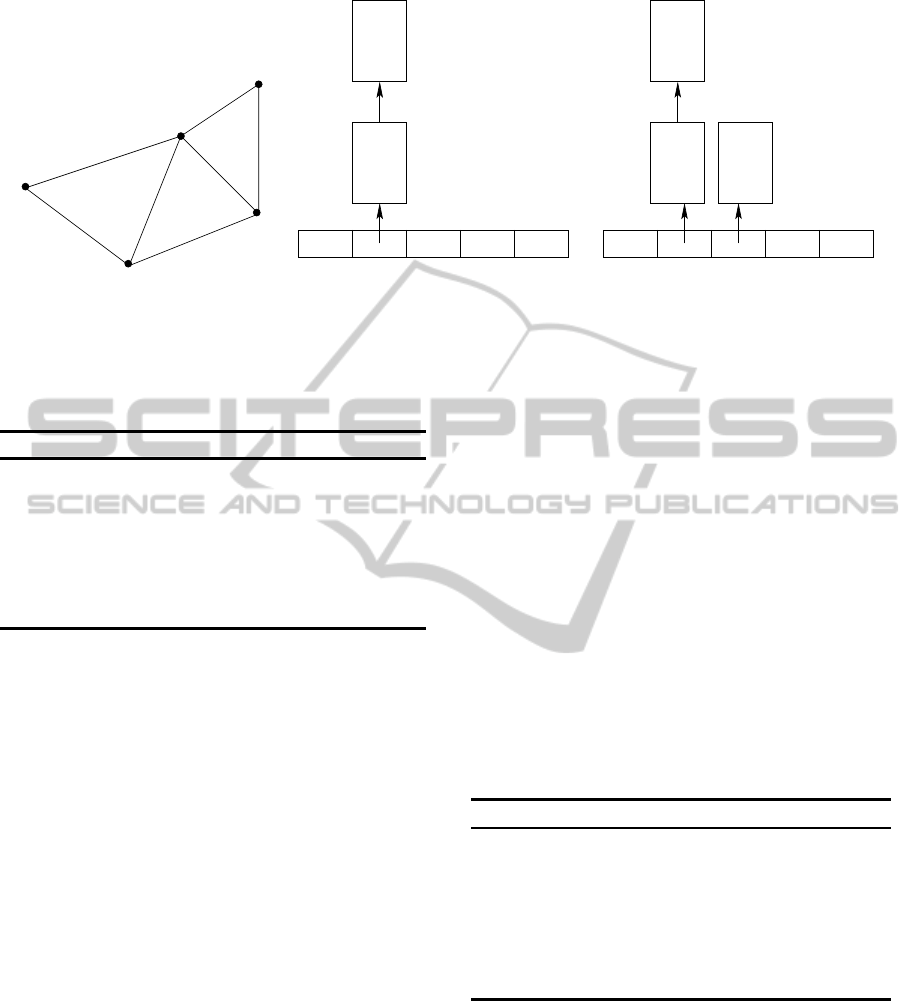
s
v
3
v
1
v
2
v
3
2
1
1
5
4
4
4
(a) graph extracted from a triangular
mesh.
b=s
2 4 6 8 10
v
1
v
2
d=4
b=s
d=3
0
(b) data structure after removing s
from the second bucket and inserting
v
1
and v
2
.
d=5
2 4 6 8 10
v
1
v
2
b=
v
3
v
2
b=
v
4
b=s
d=4
d=4
0
(c) data structure after removing v
2
from the second bucket and inserting v
3
and v
4
.
Figure 1: Illustration of the removal and insertion operations for a specific graph. d denotes the distance from the source
vertex s and b is a pointer to the previous vertex in the path.
Algorithm 4: Function DecreaseKey(Q, v).
j ←index of the bucket currently containing v
i ←⌊d(s,v)/w⌋
// compute the index of
the new bucket for
v
bucket
j
← bucket
j
− {v}
// remove
v
from bucket
j
bucket
i
← bucket
i
∪ {v}
// insert
v
into
bucket
i
as a fraction of the maximum edge size (used as cost
for Dijkstra’s algorithm), whereas n is initially set to
a constant.
After the first shortest paths computation, we re-
fine the input parameters by decreasing the bucket
width w in order to reduce the number of elements
in each bucket and hence also the number of compar-
isons required to find a minimum vertex in a bucket.
However, there is a trade-off between the sizes of w
and n. In order to avoid the overhead of visiting too
many buckets, which would happen if we reduced the
bucket width indefinitely, we limit w to be no less than
a constant that depends on the mesh at hand. The
principle behind this idea is that the number of com-
parisons decreases by indirectly setting the maximum
number of elements in each bucket according to the
input data since the variation of edge lengths is mesh
dependent.
4 EXPERIMENTAL RESULTS
In this section, we show results comparing the pro-
posed approach and other methods for implementing
the queue employed by Dijkstra’s algorithm. The re-
sults were obtained on a standard PC featuring an
Intel
R
Core 2 T200 processor, 2 Gbytes of RAM, run-
ning Windows
R
XP operating system.
The parameters used in the experiments are the
following: n = 5000 and the fraction of the maximum
edge size is set to w = 1/c, where c is initially equal to
100. After each distance computation, c is increased
by 100 if the average number of vertices per bucket in
the previous iteration is greater than 64.
Table 1 lists the models used in the experiments
as well as their numbers of vertices, edges and faces.
To obtain realistic results, we chose a set of models so
that the number of vertices range from few thousands
to over a million.
Table 1: Models used in our experiments.
Model Vertices Edges Faces
Bunny 35,947 105,396 69,451
Armadillo 172,974 527,916 354,944
Virgin 252,470 752,468 500,000
Hand 327,323 981,987 654,666
Dragon 437,645 1,309,057 871,414
Happy Buddha 543,652 1,631,366 1,087,716
Gargo 863,210 2,589,628 1,726,420
Blade 882,954 2,648,340 1,765,388
Amphora 1,317,152 3,950,260 2,633,110
Table 2 shows the number of buckets, average
number of elements per bucket and the standard de-
viation computed for each model. According to the
standard deviation, it is possible to observe that the
number of elements per bucket is almost constant,
which leads to a very small number of comparisons
performed by the function ExtractMin(Q).
Table 3 relates the actual number of comparisons
performed by the proposed method (second column)
with the values of E +V and E +V log
2
V. The num-
FasterApproximationsofShortestGeodesicPathsonPolyhedraThroughAdaptivePriorityQueue
375
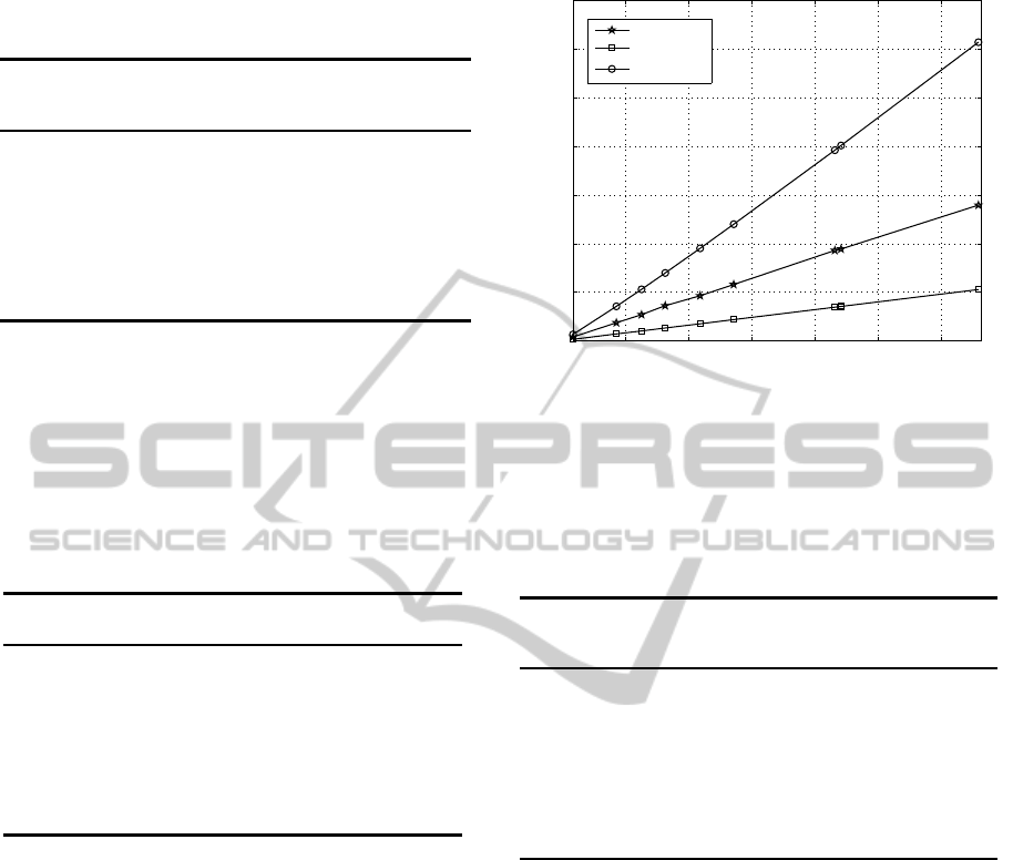
Table 2: Number of buckets, average number of elements
per bucket and its standard deviation computed for each
model used in the experiments.
Model Number of Average Number Standard
Buckets of Elements per Deviation
Bucket
Bunny 55,077 1.438 0.719
Armadillo 120,562 1.999 1.197
Virgin 186,696 1.939 1.177
Hand 290,708 2.122 1.409
Dragon 298,464 1.933 1.164
Happy Buddha 368,808 1.962 1.209
Gargo 632,312 2.032 1.311
Blade 691,346 1.939 1.195
Amphora 933,554 1.888 1.105
ber of comparisons includes the number of edges, ver-
tices and buckets visited during the entire execution of
Dijkstra’s algorithm.
Table 3: Number of comparisons performed by our method
and the expected number of comparisons according to dif-
ferent time complexities. E +V log
2
V is the expected num-
ber of comparisons to Dijkstra’s algorithm using Fibonacci
heap. V and E represent the number of vertices and edges
in the graph, respectively.
Model Number of E +V E +V log
2
V
Comparisons
Bunny 383,427 141,343 649,402
Armadillo 1,850,280 700,890 3,537,697
Virgin 2,682,909 1,004,938 5,283,232
Hand 3,604,024 1,309,310 6,978,660
Dragon 4,632,881 1,746,702 9,510,262
Happy Buddha 5,786,322 2,175,018 11,989,200
Gargo 9,291,953 3,452,838 19,611,569
Blade 9,437,125 3,531,294 20,088,428
Amphora 13,955,707 5,267,412 30,726,630
According to experimental results shown in Fig-
ure 2, the method proposed here achieves a number of
comparisons between E + V logV (due to Fibonacci
heap) and E +V (that is, linear on the number of ver-
tices and edges).
Table 4 shows a comparison between the differ-
ent implementations of the priority queue used in
Dijkstra’s algorithm. We compare four methods: a
quadratic array-based one; a Fibonacci heap; and our
proposed method based on an adaptive bucketing-
based heap.
Figure 3 displays the models used in our experi-
ments to solve the single source, all destination prob-
lem. In the results, we use hot-to-cold color ramp,
where blue is chosen for the low values of distance,
green for middle values and red for high values. For
example, on the Bunny, Figure 3(f), the source vertex
is on its right ear while its left ear is green since the
paths must lie on the surface. Also, the tail is red since
it is the farthest body part from the source vertex.
2 4 6 8 10 12
x 10
5
0
0.5
1
1.5
2
2.5
3
3.5
x 10
7
number of vertices
number of comparisons
bucketing
V + E
E + V log
2
V
Figure 2: Graph showing the growth behavior of the number
of comparisons performed by the proposed method (buck-
eting) and of the functions E +V and E +V log
2
V.
Table 4: Time comparison between the various priority
queue implementations in Dijkstra’s algorithm. The results
shown are the average of 150 executions. Preprocessing is
the time required to build the graph, which is done only
once.
Model Preprocessing Array- Fibonacci Bucketing
(s) based Heap (Heap)
(s) (s) (s)
Bunny 0.140 4.453 0.109 0.035
Armadillo 0.891 - 0.622 0.156
Virgin 0.844 - 0.837 0.209
Hand 1.109 - 1.133 0.264
Dragon 1.687 - 1.514 0.397
Happy Buddha 2.141 - 1.992 0.481
Gargo 2.953 - 3.172 0.721
Blade 2.922 - 3.074 0.802
Amphora 4.609 - 4.812 1.287
According to the results shown in Table 4, the pro-
posed method achieves the best computational time
on all models considered. On average, it is nearly
four times faster than the second best (based on the
Fibonacci heap). Furthermore, the results show that
the proposed method is suitable to be used in appli-
cations requiring a large number of computations of
single source, all destination shortest geodesic paths.
Although there are no bounds that guarantee an
ε
-
approximation when directly using the original mesh
to create the graph, many applications require only a
reasonable estimate of the shortest geodesic path, pro-
vided that such estimation is achieved quickly. For
instance, by using the original mesh of the Bunny
model, our method is able to approximate more than
28 single source, all destination shortest geodesic
paths per second, while the Fibonacci heap-based
method would compute no more than 10.
VISAPP2015-InternationalConferenceonComputerVisionTheoryandApplications
376
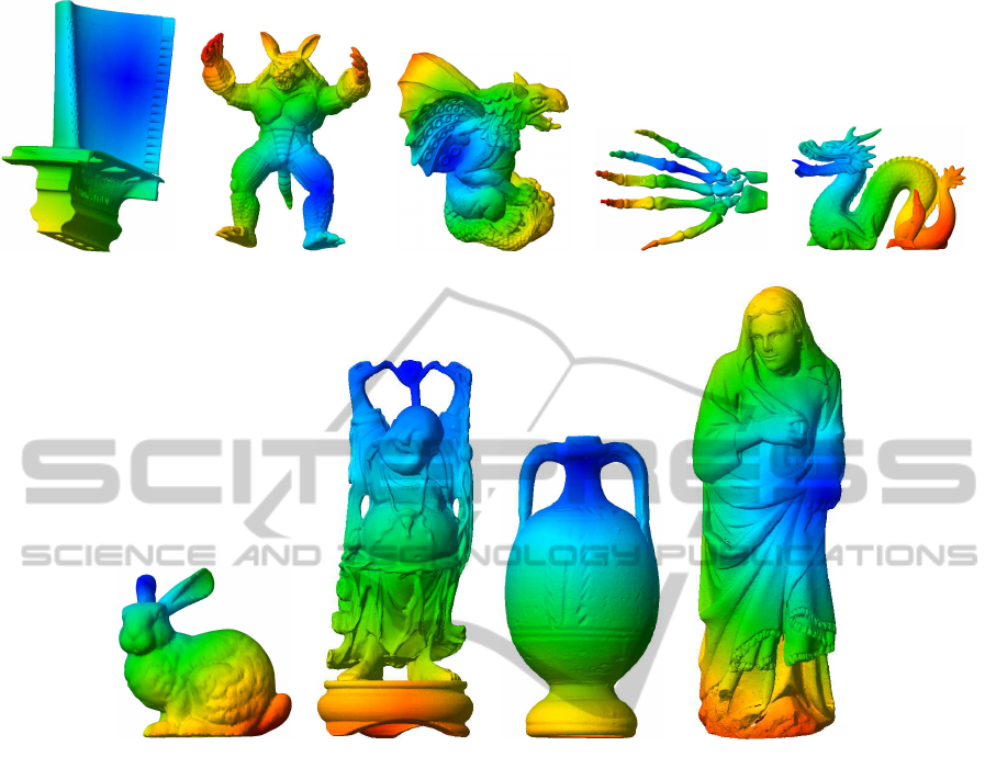
(a) Blade (b) Armadillo (c) Gargo (d) Hand (e) Dragon
(f) Bunny (g) Happy Buddha (h) Amphora (i) Virgin
Figure 3: Models used in our experiments to compute approximations of the shortest geodesic paths.
5 CONCLUSIONS
Several application areas, such as robotics, medi-
cal imaging, terrain navigation and computational
geometry, benefit from the computation of shortest
geodesic paths, which can be stated as finding the
shortest path between two points on the surface of a
polyhedron.
In this work, we propose the use of a priority
queue based on a bucketing data structure in Di-
jkstra’s algorithm for computing approximations of
shortest geodesic paths. The experiments show that
our approach is fast and can be used in applications
that require approximations for the geodesic distance.
ACKNOWLEDGEMENTS
This research was supported by grants from:
FAPESP, FAPEMIG, CAPES, CNPq #477692/2012-
5, #307113/2012-4 and #477457/2013-4.
REFERENCES
Agarwal, P., Har-Peled, S., and Karia, M. (2002). Comput-
ing Approximate Shortest Paths on Convex Polytopes.
Algorithmica, 33:227–242.
Ahuja, R. K., Mehlhorn, K., Orlin, J. B., and Tarjan, R. E.
(1990). Faster Algorithms for the Shortest Path Prob-
lem. Journal of the ACM, 37:213–223.
Aleksandrov, L., Lanthier, M., Maheshwari, A., and Sack,
J.-R. (1998). An
ε
-approximation for Weighted Short-
est Paths on Polyhedral Surfaces. In Proc. 6th Scan-
dinavian Workshop on Algorithm Theory - Lecture
Notes in Computer Science, volume 1432, pages 11–
22.
Aleksandrov, L., Maheshwari, A., and Sack, J.-R.
(2005). Determining Approximate Shortest Paths on
Weighted Polyhedral Surfaces. Journal of the ACM,
52(1):25–53.
Barbehenn, M. (1998). A Note on the Complexity of Di-
jkstra’s Algorithm for Graphs with Weighted Vertices.
IEEE Transactions on Computers, 47:263.
Bose, P., Maheshwari, A., Shu, C., and Wuhrer, S. (2011).
FasterApproximationsofShortestGeodesicPathsonPolyhedraThroughAdaptivePriorityQueue
377

A Survey of Geodesic Paths on 3D Surfaces. Compu-
tational Geometry, 44(9):486–498.
Bronstein, A., Bronstein, M., Kimmel, R., Mahmoudi, M.,
and Sapiro, G. (2010). A Gromov-Hausdorff Frame-
work with Diffusion Geometry for Topologically-
Robust Non-rigid Shape Matching. International
Journal of Computer Vision, 89:266–286.
Chen, J. and Han, Y. (1990). Shortest Paths on a Polyhe-
dron. In Proc. 6th Annual Symposium on Computa-
tional Geometry, pages 360–369.
Cormen, T. H., Leiserson, C. E., Rivest, R. L., and Stein,
C. (2001). Introduction to Algorithms. MIT Press and
McGraw-Hill, second edition.
Dijkstra, E. W. (1959). A Note on Two Problems in Con-
nection with Graphs. Numerische Mathematik, 1:269–
271.
Hamza, A. B. and Krim, H. (2003). Geodesic Object Rep-
resentation and Recognition. In Proc. International
Conference on Discrete Geometry for Computer Im-
agery, volume 2, pages 378–387.
Hershberger, J. and Suri, S. (1993). Efficient Computation
of Euclidean Shortest Paths in the Plane. In Proc. 34th
Annual Symposium on Foundations of Computer Sci-
ence, pages 508–517, Palo Alto, CA, USA.
Hilaga, M., Shinagawa, Y., Kohmura, T., and Kunit, T. L.
(2001). Topology Matching for Fully Automatic Sim-
ilarity Estimation of 3D Shapes. In Proc. Conference
on Computer Graphics (SIGGRAPH), pages 203–212.
Hwang, Y. K. and Ahuja, N. (1992). Gross Motion Plan-
ning: A Survey. ACM Computer Survey, 24(3):219–
291.
Kamousi, P., Lazard, S., Maheshwari, A., and Wuhrer, S.
(2013). Analysis of Farthest Point Sampling for Ap-
proximating Geodesics in a Graph. arXiv.org.
Kanai, T. and Suzuki, H. (2001). Approximate Shortest
Path on a Polyhedral Surface and its Applications.
Computer-Aided Design, 33(11):801–811.
Kapoor, S. (1999). Efficient Computation of Geodesic
Shortest Paths. In Proc. 31st Annual ACM Symposium
on Theory of Computing, pages 770–779, Atlanta-GA,
USA.
Kimmel, R. and Sethian, J. A. (1998). Computing Geodesic
Paths on Manifolds. Proc. National Academy of Sci-
ences of the United States of America, 95(15):8431–
8435.
Li, Z., Jin, Y., Jin, X., and Ma, L. (2012). Approximate
Straightest Path Computation and its Application in
Parameterization. The Visual Computer, 28(1):63–74.
Lozano-Prez, T. and Wesley, M. A. (1979). An Algorithm
for Planning Collision-Free Paths among Polyhedral
Obstacles. Communications of the ACM, 22(10):560–
570.
Mitchell, J. S. B., Mount, D. M., and Papadimitriou, C. H.
(1987). The Discrete Geodesic Problem. SIAM Jour-
nal on Computing, 16(4):647–668.
Mount, D. (1985). On Finding Shortest Paths in Con-
vex Polyhedra. Technical Report 1495, University of
Maryland, Baltimore, USA.
Mount, D. (1986). Storing the Subdivision of a Polyhedral
Surface. In Second Annual Symposium on Computa-
tional Geometry, pages 150–158.
Novotni, M. and Klein, R. (2002). Computing Geodesic
Distances on Triangular Meshes. In Proc. 10th Inter-
national Conference in Central Europe on Computer
Graphics, pages 341–347.
Onclinx, V., Lee, J., Wertz, V., and Verleysen, M. (2010).
Dimensionality Reduction by Rank Preservation. In
International Joint Conference on Neural Networks,
pages 1 –8.
O’Rourke, J., Suri, S., and Booth, H. (1985). Shortest Paths
on Polyhedral Surfaces. In Proc. 2nd Symposium of
Theoretical Aspects of Computer Science, pages 243–
254.
Papadimitriou, C. H. (1985). An Algorithm for Shortest-
Path Motion in Three Dimensions. Information Pro-
cessing Letters, 20:259–263.
Peyr´e, G., P´echaud, M., Keriven, R., and Cohen, L. D.
(2010). Geodesic Methods in Computer Vision and
Graphics. Foundations and Trends in Computer
Graphics and Vision, 5:197–397.
Rabin, J., Peyr´e, G., and Cohen, L. D. (2010). Geodesic
Shape Retrieval via Optimal Mass Transport. In Pro-
ceedings of the 11th European conference on Com-
puter Vision: Part V, pages 771–784, Heraklion,
Crete, Greece. Springer-Verlag.
Sharir, M. and Schorr, A. (1986). On Shortest Paths in
Polyhedral Spaces. SIAM Journal on Computing,
15(1):193–215.
Surazhsky, V., Surazhsky, T., Kirsanov, D., Gortler, S. J.,
and Hoppe, H. (2005). Fast Exact and Approximate
Geodesics on Meshes. ACM Transactions on Graph-
ics, 24(3):553–560.
Tenenbaum, J. B., de Silva, V., and Langford, J. C. (2000).
A Global Geometric Framework for Nonlinear Di-
mensionality Reduction. Science, 290:2319–2323.
Varadarajan, K. R. and Agarwal, P. K. (2000). Approximat-
ing Shortest Paths on a Nonconvex Polyhedron. SIAM
Journal on Computing, 30(4):1321–1340.
Wang, K., Lavoue, G., Denis, F., and Baskurt, A. (2008). A
Comprehensive Survey on Three-Dimensional Mesh
Watermarking. IEEE Transactions on Multimedia,
10(8):1513–1527.
Ying, X., Wang, X., and He, Y. (2013). Saddle Ver-
tex Graph (SVG): A Novel Solution to the Discrete
Geodesic Problem. ACM Transactions on Graphics,
32(6):170:1–170:12.
Zigelman, G., Kimmel, R., and Kiryati, N. (2002). Tex-
ture Mapping Using Surface Flattening via Multidi-
mensional Scaling. IEEE Transactions on Visualiza-
tion and Computer Graphics, 8(2):198–207.
VISAPP2015-InternationalConferenceonComputerVisionTheoryandApplications
378
