Breast Tissue Characterization in X-Ray and Ultrasound Images using
Fuzzy Local Directional Patterns and Support Vector Machines
Mohamed Abdel-Nasser
1
, Domenec Puig
1
, Antonio Moreno
1
, Adel Saleh
1
, Joan Marti
2
, Luis Martin
3
and Anna Magarolas
3
1
Department of Computer Engineering and Mathematics, Rovira i Virgili University, Tarragona, Spain
2
Dept. of Electronics, Computer Engineering and Automatics, University of Girona, Girona, Spain
3
Hospital Universitari Joan XXIII de Tarragona, Tarragona, Spain
Keywords:
Feature Extraction, Fuzzy Logic, Classification, X-ray Images, Ultrasound Images.
Abstract:
Accurate breast mass detection in mammographies is a difficult task, especially with dense tissues. Although
ultrasound images can detect breast masses even in dense breasts, they are always corrupted by noise. In this
paper, we propose fuzzy local directional patterns for breast mass detection in X-ray as well as ultrasound
images. Fuzzy logic is applied on the edge responses of the given pixels to produce a meaningful descriptor.
The proposed descriptor can properly discriminate between mass and normal tissues under different conditions
such as noise and compression variation. In order to assess the effectiveness of the proposed descriptor, a
support vector machine classifier is used to perform mass/normal classification in a set of regions of interest.
The proposed method has been validated using the well-known mini-MIAS breast cancer database (X-ray
images) as well as an ultrasound breast cancer database. Moreover, quantitative results are shown in terms of
area under the curve of the receiver operating curve analysis.
1 INTRODUCTION
Breast cancer is considered as one of the most dan-
gerous cancers that attacks women (DeSantis et al.,
2014). Early detection of breast cancer yields a reduc-
tion in mortality. Mammographies are the most effec-
tive method of breast cancer screening. In a mam-
mography, each breast is compressed using compres-
sion plates, then it is X-rayed from top to bottom or
by angle. In turn, Sonographies are safer and pain-
less, and they generate real time images of the inside
of the breast using ultrasound waves. Breast density
is one of the main failure factors of mammographies
because dense tissues may hide some tumour regions.
Breast density represents the relative amounts
of fibroglandular and fat tissue in a woman
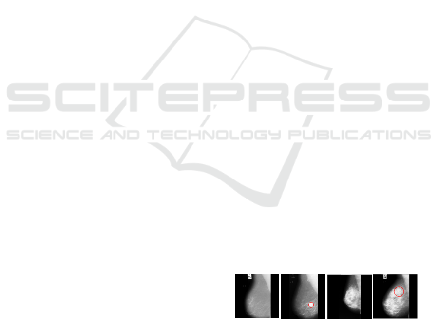
breast (Lokate et al., 2010). The well-known mini-
MIAS breast cancer database (Suckling et al., 1994)
classifies the breast density into three categories:
fatty, fatty-glandular and dense glandular (see Fig. 1).
Dense breasts have more glandular and fibrous tis-
sues, and they appear white in the mammogram.
Therefore, they hide cancer regions, which also usu-
ally appear white in mammograms. In turn, fatty
breasts have more fatty tissues and they can be seen
grey in mammograms. Thus, it is easy to detect can-
cer in fatty breasts. Indeed, sonographies are superior
to mammographies in their ability to detect abnormal-
ities in the dense breasts. Sonographies have become
an important assistant to mammographies in breast
cancer detection. They cannot replace a mammogram
for breast screening, but they can provide more help
to physicians.
(a)
(b)
(c)
(d)
Figure 1: Mammogram examples in the mini-MIAS breast
cancer database. Fatty mammogram containing: (a) normal
and, (b) mass tissue (see the red circle). Dense mammogram
containing: (c) normal and, (d) mass tissue (mass detection
is not evident in this case).
Numerous computer aided diagnosis (CAD) sys-
tems have been proposed for breast mass detection
with X-ray or ultrasound images. A breast mass CAD
system usually consists of two main steps: feature
extraction and classification. A comparison of vari-
ous texture analysis methods for breast mass detec-
tion in X-ray images is presented in (Abdel-Nasser
et al., 2014). For instance, Oliver et al. used the his-
togram of the local binary pattern (LBP) to reduce
387
Abdel-Nasser M., Puig D., Moreno A., Saleh A., Marti J., Martin L. and Magarolas A..
Breast Tissue Characterization in X-Ray and Ultrasound Images using Fuzzy Local Directional Patterns and Support Vector Machines.
DOI: 10.5220/0005264803870394
In Proceedings of the 10th International Conference on Computer Vision Theory and Applications (VISAPP-2015), pages 387-394
ISBN: 978-989-758-089-5
Copyright
c
2015 SCITEPRESS (Science and Technology Publications, Lda.)

the number of false positives of breast mass detec-
tion (Oliver et al., 2007). They used a support vec-
tor machine (SVM) for classification. Unfortunately,
LBP may assign the same pattern to a pixel in a tu-
morous region and another pixel in a normal dense
tissue, yielding a noticeable percentage of false detec-
tions. The histogram of oriented gradient (HoG) has
also been used for breast mass detection (Pomponiu
et al., 2014). HoG is used to train a SVM classifier.
The cell size and the number of cells per block need to
be optimized. If an unsuitable block size is used, the
same HoG descriptor may be produced for a normal
block and a tumorous block in dense mammograms
leading to high number of false detections.
In turn, a discussion of the approaches used in ul-
trasound breast images CAD stages and a summary
of their advantages and disadvantages are presented
in (Shi et al., 2010). A breast cancer CAD system
based on a fuzzy support vector machine is developed
in (Shi et al., 2010) to automatically detect masses
in ultrasound images. Moreover, fuzzy local binary
patterns (FLBP) are proposed in (Keramidas et al.,
2011). FLBP incorporate fuzzy logic in the repre-
sentation of the local patterns in ultrasound images.
FLBP are extracted from a set of regions of interest
(ROIs) acquired from thyroid ultrasound images, and
then a SVM classifier is used to classify them into
nodule or non-nodule classes.
Noise, breast density and the variation in breast
compressions yield a fuzzy appearance of the breast
tissues. Unfortunately, the literature shows no con-
sensus on an optimal feature set for mass/normal
breast tissue classification, which means that the
methods proposed in the literature don’t produce a
complete characterization of different tissues in breast
images, yielding a high number of false positives
(ROIs interpreted by a CAD system as abnormal
when they are actually normal).
In this paper, the proposed work focuses on the
feature extraction sub-task of breast cancer CAD sys-
tem by proposing the fuzzy local directional pattern
(FLDP) for characterizing breast tissues. The ratio-
nale behind the use of fuzzy logic is to compensate
the uncertainty of the visual appearance of breast tis-
sues due to noise, breast density and the variation
in breast compressions. FLDP describes the shapes,
margins, spots, edges, corners, junctions and other
structures of different tissues in a breast region. FLDP
is evaluated with mass/normal classification of ROIs
extracted from X-ray, and ultrasound images.
The rest of this paper is organized as follows. Sec-
tion 2 explains the related descriptors as well as the
proposed descriptor. Section 3 explains the use of
the proposed descriptor in breast tissue classification.
Section 4 includes the experimental results and dis-
cussion. Section 5 summarises our work, and sug-
gests some lines of future work.
2 FUZZY LOCAL DIRECTIONAL
PATTERN
This section comments the most related descriptors
and explains in detail the proposed descriptor.
2.1 Related Descriptors
In (Oliver et al., 2007), LBP is used as a texture de-
scriptor for reducing the number of false positives in
breast cancer detection. The original LBP operator
compares the intensity values of the eight neighbors
of a 3 × 3 neighborhood around a pixel with the in-
tensity value of this pixel. The corresponding bit of
a neighbor pixel that has a higher intensity than the
central pixel is set to 1 otherwise it is set to 0. Thus,
each pixel is represented by 8 bits as shown in (Ojala
et al., 2002). Thus, LBP depends on the intensity dif-
ference of the pixels that is very sensitive to noise and
to illumination changes.
The robust local binary pattern (RLBP) is pro-
posed in (Chen et al., 2013) to correct the non-
uniform patterns in the LBP binary codes to reduce
the effect of noise. Chen’s method partitioned each
8-bit LBP binary code in sets of three consecutive
bits. If 010 or 101 are found in the generated codes,
they are replaced by 000 or 111 respectively. Chen’s
method converts a natural non-uniform pattern into
a uniform pattern, which leads to a distortion in the
overall description, because any wrong correction af-
fects the final histogram.
Fig. 2 presents an example of the calculation of
LBP codes for two different pixels, A and B: pixel A
lays in a tumorous region, while pixel B belongs to a
normal region. Although the two pixels are in com-
pletely different regions, LBP assigns the same binary
code 00000000 to both of them, causing a dilemma
in the classification stage (RLBP calculates the same
codes).
The local directional pattern (LDP) is a robust
grey scale texture descriptor that encodes the edge
responses in a local neighbourhood. In this way,
LDP reduces the reliance on the intensity difference
used in LBP to be more robust against noise and
changes in illumination. LDP computes the edge re-
sponses in eight directions by using compass Kirsch
masks (Gonzalez and Woods, 2002). Jabid et al. pro-
posed to set the top k responses positions to ’1’ and
the other directions to ’0’ generating a 8-bit code for
VISAPP2015-InternationalConferenceonComputerVisionTheoryandApplications
388
each pixel (Jabid et al., 2010). Fig. 2 shows an ex-
ample of the calculation of LDP codes. LDP assigns
00101001 to pixel A and 10100001 to pixel B. Al-
though LDP generates different codes, the reliance on
only the top three responses leads to a loss of infor-
mation about a local neighbourhood.
In addition, the local directional number (LDN)
is proposed in (Ramirez Rivera et al., 2013). In
LDN, the edge responses are computed in eight di-
rections by convolving the derivative-Gaussian masks
with the original image. In (Ramirez Rivera et al.,
2013), the derivative of a skewed Gaussian is used to
create an asymmetric compass mask in order to get
more robust edge responses against noise. The edge
responses (m
0
,m
45
,m
90
,m
135
,m
180
,m
225
,m
270
,m
315
)
were assigned to the location codes (000, 001, 010,
011, 100, 101, 110, 111), respectively. The LDN de-
scriptor concatenates the location codes of the highest
positive and the smallest negative responses to pro-
duce the final 6-bit descriptor of each pixel. Fig. 2
shows an example of the calculation of LDN codes.
LDN can distinguish between pixel A and B by as-
signing different codes 100111 and 010111, respec-
tively. However, LDN may lose information about the
neighbors in a certain neighbourhood because only
the minimum and maximum responses are consid-
ered.
Finally, the modified local directional pattern
(MLDP) is proposed in (Mohamed et al., 2014) to
improve the robustness of optical flow estimation.
MLDP encodes the edge responses computed by us-
ing the Kirsch compass masks based on a Gaussian
filter. In Fig. 2, MLDP assigns 10000011 to pixel A
and 10001011 to pixel B.
92 89 90
91 222 220
88 215 213
47 39 40
46 55 52
46 51 50
-1118 -1126 -102
-1126 890
-142 834 1890
-27 -75 -35
29 53
-19 13 61
c2
c4
c1
c3
c6c5 c7
c0
c6c5 c7
c2 c1
c3
c0
c4
m
0
m
270
m
135
m
90
m
315
m
45
m
225
m
180
m
270
m
315
m
225
m
135
m
90
m
45
m
0
m
180
A
B
Edge Response
Edge Response
3x3 neighbourhood
3x3 neighbourhood
B
LBP: 00000000
RLBP: 00000000
LDP: 10100001
LDN: 010111
MLDP: 10001011
A
LBP: 00000000
RLBP: 00000000
LDP: 00101001
LDN: 100111
MLDP: 10000011
Figure 2: The binary codes generated with LBP, RLBP,
LDP, LDN and MLDP for pixel A (tumorous) and pixel B
(normal), c
0
− c
7
are the Kirsch compass masks presented
in Fig. 4.
2.2 Proposed Descriptor
After identifying the main problems of the related de-
scriptors, we propose FLDP as a texture descriptor for
breast tissue characterization. FLDP describes a given
pixel through its edge responses. The edge responses
ER of each pixel are computed using the Kirsch com-
pass masks (see Fig.4). Given a certain pixel, its eight
edge responses ER can be defined as such:
ER =
{
ER
0
,ER
1
,...ER
7
}
∈ R
8
(1)
Let A be the set of the ER greater than zero, and B the
set of the ER smaller than zero:
A ≡
ER
i
| 0 ≤ i ≤ 7, ER
i
≥ 0
(2)
B ≡ ER − A ≡
ER
i
| 0 ≤ i ≤ 7, ER
i
< 0
(3)
In crisp approaches, a hard threshold is used to deter-
mine the prediction of each variable. In turn, fuzzy
logic allows the use of a membership function to de-
termine the class of each variable. In the fuzzification
process, each input variable is mapped to its corre-
sponding fuzzy variable according to a set of fuzzy
rules (Zadeh, 1965). A and B can be defined as two
fuzzy sets
∼
A and
∼
B, where
∼
A contains the positive
edge responses, and
∼
B contains the negative edge re-
sponses. The fuzzy sets
∼
A and
∼
B can be expressed as
such:
∼
A ≡ {
ER
i
,µ
+
(ER
i
)
| 0 ≤ i ≤ 7, µ
+
(ER
i
) ≥ µ
−
(ER
i
)}
(4)
∼
B ≡ {
ER
i
,µ
−
(ER
i
)
| 0 ≤ i ≤ 7, µ
−
(ER
i
) > µ
+
(ER
i
)}
(5)
1
-α
α
0
Membership value
ER
μ
(
ER
1
)
μ
(
ER
1
)
ER
1
0.5
μ
+
(
ER
)
μ
-
(
ER
)
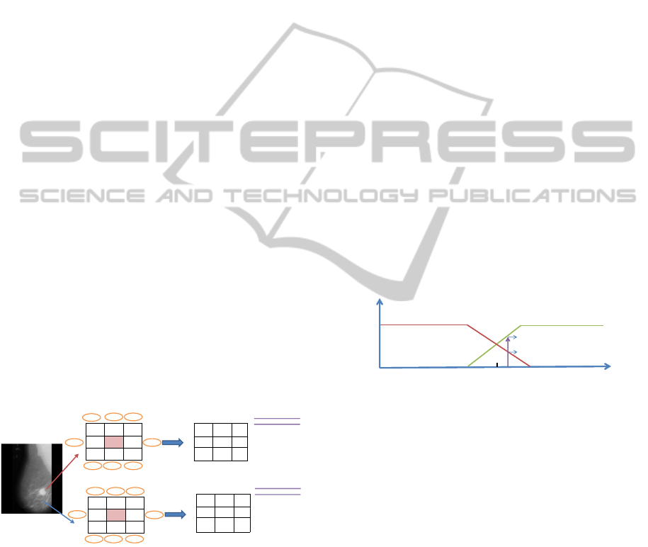
Figure 3: Linear membership functions, the green curve
represents the membership function of the positive fuzzy
set, whereas the blue curve represents the membership func-
tion of the negative fuzzy set.
Given an edge response, its degree of membership
to these fuzzy sets can be computed. We used a linear
function in order to calculate the degree of each edge
response ER
i
to be negative, or the degree of each ER
i
to be positive (see Fig. 3). Let µ
+
define the degree
of each ER
i
to be positive:
µ
+
(ER
i
) =
0 if ER
i
< −α
0.5 +ER
i
/2α if −α ≤ ER
i
≤ α
1 if ER
i
> α,
(6)
where α is a threshold. In addition, µ
−
defines the
degree of each ER to be negative:
µ
−
(ER
i
) = 1 − µ
+
(ER
i
) (7)
Given the vector ER of a certain pixel, the degree of
membership of each edge response to the positive and
BreastTissueCharacterizationinX-RayandUltrasoundImagesusingFuzzyLocalDirectionalPatternsandSupportVector
Machines
389

negative fuzzy sets can be computed. Each edge re-
sponse ER
i
may belong to one of the following cate-
gories:
a) µ
+
(ER
i
) = 1, µ
−
(ER
i
) = 0, [ER
i
≥ α]
b) µ
+
(ER
i
) = 0, µ
−
(ER
i
) = 1, [ER
i
≤ −α]
c) µ
+
(ER
i
) > 0, µ
−
(ER
i
) > 0, [−α < ER
i
< α]
Let us define the subset of edge responses that be-
long to category c:
ER
0
=
ER
i
| 0 ≤ i ≤ 7, µ
+
(ER
i
) > 0, µ
−
(ER
i
) > 0
(8)
where ER
0
⊆ ER. ER contains eight edge responses,
and ER
0
is the subset of those edge responses in the
fuzzy interval [−α,α]. For a given pixel, let us de-
fine the number of the elements in the subset ER
0
as
k =
ER
0
, 0 ≤ k ≤ 8. Given ER and ER
0
of a certain
pixel, 2
k
different 8-bits binary codes can be built as
follows:
• If an edge response ER
i
belongs to category
a,
µ
+
(ER
i
) = 1, µ
−
(ER
i
) = 0
, then all the 2
k
codes will have ’1’ in position i of the binary code.
• If an edge response ER
i
belongs to category
b,
µ
+
(ER
i
) = 0, µ
−
(ER
i
) = 1
, then all the 2
k
codes will have ’0’ in position i of the binary code.
• The remaining k edge responses belong to cate-
gory c, and the k bits associated to these k edge
responses will be assigned different codes from
000...0
| {z }
k- bits
to 111 ...1
| {z }
k- bits
in the 2
k
binary codes to be
built.
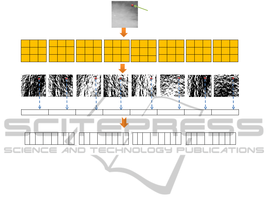
Fig. 4 presents an example of the calculation of FLDP
with the threshold α = 100. Both of ER
2
= −10 and
ER
3
= 30 are located in the fuzzy interval [−α,α]. In
this example, k = 2, so 2
2
FLDP codes are computed
as follows:
• ER
0,1,6
belong to category b (’0’ will be assigned
to the associated positions).
• ER
4,5,7
belong to category a (’1’ will be assigned
to the associated positions).
• ER
2,3
belong to category c, consequently, four 2-
bit combinations: ’00’, ’10’, ’01’ and ’11’, are
assigned to the associated positions of ER
2,3
in
the four 8-bits codes.
The critical parameter of FLDP is the selection of the
proper value of the threshold α. The role of α in the
generation of FLDP codes can be explained as fol-
lows:
• If α is big, most of the edge responses will belong
to category c, and the number of the fuzzy cases
(i.e. k) for each pixel will be high (in the limit,
256).
• If α is small, most of the edge responses will be-
long to categories a and b, and the number of
fuzzy cases for each pixel will be low (in the limit,
1).
• If α = 0, the calculations will be performed in the
crisp space, i.e. there is no fuzzy interval. Con-
sequently, the crisp sets of Eq.2 and Eq.3 will be
used to calculate the binary codes. If the edge re-
sponse is positive, ’1’ will be assigned in its as-
sociated position in the binary code. If the edge
response is negative, ’0’ will be assigned in its as-
sociated position in the binary code.
In order to find the best value of α, a grid search pro-
cedure is used. In this paper, α is allowed to vary in
the range of 10
2
≤ α ≤ 10
3
.
For each pixel, a set of m 8-bits binary codes
(1 ≤ m ≤ 256) having values between 0 and 255 is
generated. Each of these 8-bits codes C = [c
0
c
1
...c
7
]
may be assigned a certain weight w
c
, depending on
the degree of the membership function of the asso-
ciated edge response to the positive or negative fuzzy
sets (depending on whether the bit in the code is ’1’ or
’0’, respectively). Given a binary code C, its weight
w
c
can be computed as follows:
w
c
(C) =
7
∏
i=0
c
i
.µ
+
(ER
i
) +(1 − c
i
).µ
−
(ER
i
) (9)
Given a certain pixel with a set of edge responses from
which 2
k
codes have been generated, it can be proved
that the addition of the weights of these 2
k
codes is 1.
Calling back the example of Fig. 4, we can use Eq. 6
and Eq. 7 to calculate the degree of membership of
ER
2
and ER
3
to the positive and negative fuzzy sets as
follows: µ
+
(ER
2
)=µ
+
(−10)=0.45, µ
−
(ER
2
)=0.55,
µ
+
(ER
3
)=µ
+
(30)=0.65, µ
−
(ER
3
)=0.35. The
weight of each fuzzy code can be calculated
using Eq.9, w
c
(C
1
)=0.55 × 0.35 = 0.1925,
w
c
(C
2
)=0.35 ×0.45 = 0.1575, w
c
(C
3
)=0.55 ×0.65 =
0.3575, w
c
(C
4
)=0.45 × 0.65 = 0.2925. It
is clear that the addition of the weights
(0.1925 + 0.1575 + 0.3575 + 0.2925) of the fuzzy
codes of the pixel given in Fig. 4 equals 1.
The codes associated to a pixel may be repre-
sented graphically in a histogram in which the x-axis
is the decimal value of each code (0-255) and the y-
axis is the weight associated to that code. Given a
grey level ROI, the complete FLDP histogram is com-
puted by adding the weights of all the pixels in the
input ROI (Ahonen and Pietik
¨
ainen, 2007).
VISAPP2015-InternationalConferenceonComputerVisionTheoryandApplications
390
5 -3 -3
5 0 -3
5 -3 -3
-3 -3 -3
-3 0 -3
5 5 5
5 5 5
-3 0 -3
-3 -3 -3
-3 -3 -3
-3 0 5
-3 5 5
-3
-3
-3
5 0 -3
5 5 -3
5 5 -3
5 0 -3
-3 -3 -3
-3 5 5
-3 0 5
-3 -3 -3
-3 -3 5
-3 0 5
-3 -3 5
convolving with Kirsch Compass masks
Pixel under
processing
eight edge responses are calculated per each pixel
-1000 -800 -10 30 200 700 -780 900
apply fuzzy threshold, α=100
0
1
0
1
0
μ
-
0
μ
-
1
0
1
1
0
1
1
1
0
1
0
1
0
μ
-
1
μ
+
1
0
1
1
0
1
1
1
0
1
0
1
1
μ
+
0
μ
-
1
0
1
1
0
1
1
1
0
1
0
1
1
μ
+
1
μ
+
1
0
1
1
0
1
1
1
C
1
=00001101
C
2
=00011101C
3
=00101101
C
4
=00111101
ER
0
ER
1
ER
2
ER
7
0 1 2 3 4 5 6 7
0 1 2 3 4 5 6 7
0 1 2 3 4 5 6 7
0 1 2 3 4 5 6 7
ER
3
ER
4
ER
5
ER
6
Figure 4: Example of the calculation of FLDP codes.
3 BREAST TISSUE
CLASSIFICATION
In this paper, we put forward the claim that FLDP
produces good characterization for different tissues in
breast images. Given a set of normal and mass ROIs,
FLDP is extracted from each ROI and fed to a SVM
classifier. Then, the trained model is used to classify
a query ROI as mass or normal.
3.1 Classification Stage
SVM is a supervised learning classifier that discrim-
inates between positive and negative classes by find-
ing a hyperplane that separates the classes. During the
optimization process of SVM, the training data x
i
are
mapped to a higher dimensional space using a kernel
function, K(x
i
,x
j
) = (φ
T
(x
i
).φ(x
j
)). SVM uses the
kernel trick, by which the data becomes linearly sep-
arable in the new space. The SVM classifer finds the
hyperplane with a maximum separation between the
classes in the new higher dimensional space. In the
case of a Linear SVM (LSVM) classifier, φ refers to a
dot product, whereas in a Non-Linear SVM (NLSVM)
the classifier function is formed by non-linearly pro-
jecting the training data of the input space to a feature
space of a higher dimension.
In this paper, we used a radial basis function
(RBF) as a mapping kernel, which is defined as fol-
lows:
K(x
i
,x
j
) = exp
−γkx
i
− x
j
k
2
2
, (10)
In this equation γ = 1/2σ
2
, kx
i
− x
j
k
2
2
is the squared
Euclidean distance between the two feature vectors x
i
and x
j
, and σ is a free parameter. In this paper, SVM
classifier is implemented with Matlab, and based on
libSVM library (Chang and Lin, 2011). In addition,
a grid search algorithm was performed to find the op-
timum parameters of the RBF kernel (i.e., γ and the
regularization parameter, C). In this work, we pre-
set the ranges of the grid search algorithm with steps
that equal 0.5 of the exponent. It searches for γ in the
range of 2
−5
< γ < 2
3
and C is allowed to vary in the
range of 2
−5
< C < 2
10
.
3.2 Data Sets
The mini-MIAS breast cancer database (X-ray im-
ages) is used in our experiments (Suckling et al.,
1994). It contains 332 images (1024 × 1024 pixels,
pgm format) for 116 women in MLO view. The mini-
MIAS database was created from the original MIAS
database (digitised at 50 µ pixel edge) by down-
sampling it to 200 µ pixel and clipping/padding it to
a fixed size (this step was done by the authors of the
database). The database has a ground truth (GT) pro-
vided by the radiologists and confirmed by a biopsy
BreastTissueCharacterizationinX-RayandUltrasoundImagesusingFuzzyLocalDirectionalPatternsandSupportVector
Machines
391
test (biopsy test is an analysis of a sample from a sus-
picious breast tissue under a microscope). The GT
of mini-MIAS shows the location of the abnormality,
the radius of the circle enclosing the abnormal region,
the characteristics of the background tissues and the
breast density of each image.
In addition, a set of 267 breast B-mode ultra-
sound (US) images is used. The images were col-
lected from 267 patients in UDIAT Diagnostic Centre
of Sabadell (Spain) using a Siemens ACUSON Se-
quoia C512 system 17L5 HD linear array transducer
(8.5 MHz). 104 of the images are normal and 163 im-
ages contain masses. The US database contains the
GT of the lesions that appear in the abnormal image.
Ground Truth
Region of Interest
(ROI)
Pectoral
Muscle
Labels
Background
(a)
Normal ROI
Ground Truth
Mass ROI
(b)
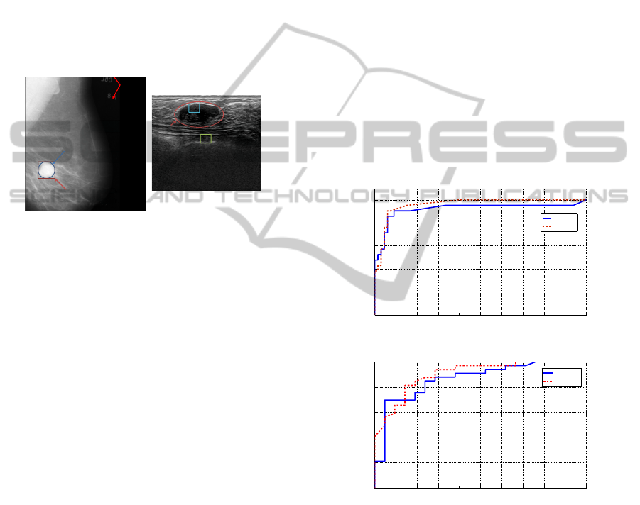
Figure 5: ROI generation using the GT of : (a) mini-MIAS,
(b) US databases.
In order to generate the ROIs we followed the pro-
cedure given in (Garc
´
ıa-Manso et al., 2013). Fig. 5(a)
presents an example of the GT of a mass region which
is the blue circle, and the ROI that is the red square
surrounding the circle. The ROIs of the normal tis-
sues were randomly selected from the normal mam-
mograms, and they were created with random sizes
ranging from the smallest to the largest size found in
the database. Fig. 5(b) presents an example of the nor-
mal and mass ROI generation in breast ultrasound im-
ages. With the mini-MIAS database, 109 mass ROIs
were extracted from the mass mammograms and 203
normal ROIs were extracted from the normal mam-
mograms. The extracted ROIs had different sizes, so
they were resized into a fixed template (in this paper,
75 × 75 pixels). With the US database, 32 × 32 pix-
els ROIs were extracted (Keramidas et al., 2011). 107
mass ROIs and 300 normal ROIs were extracted from
US images.
3.3 Evaluation
The performance of breast tissue classification using
FLDP is measured in terms of the area under the curve
(AUC) of the receiver operating curve (ROC) (Hanley
and McNeil, 1982). We used the k-fold cross vali-
dation technique to generate the training and testing
data. In this procedure, the data are partitioned into k
folds, 1/k of ROIs are used for testing and the rest of
ROIs are used for training (in this work, k=10). We
calculated the AUC valus to evaluate the performance
of FLDP with mass/normal breast tissue classification
(AUC is averaged through the cross validation pro-
cess).
4 EXPERIMENTAL RESULTS
AND DISSCUSION
Fig. 6 (a) shows the receiver operating curve of the
classification of the X-ray ROIs with LSVM and
NLSVM classifiers. The best AUC value is achieved
with the NLSVM classifiers. Fig. 6 (b) shows the
ROC of classification of the US ROIs, in which the
best result is also achieved with the NLSVM classi-
fier.
0 0.1 0.2 0.3 0.4 0.5 0.6 0.7 0.8 0.9 1
0
0.2
0.4
0.6
0.8
1
1 − specificity
sensitivity
LSVM
NLSVM
(a)
0 0.1 0.2 0.3 0.4 0.5 0.6 0.7 0.8 0.9 1
0
0.2
0.4
0.6
0.8
1
1 − specificity
sensitivity
LSVM
NLSVM
(b)
Figure 6: ROC curves of mass/normal breast tissue classifi-
cation using FLDP with (a) X-ray and (b) US datasets.
As mentioned in Section 2, the critical parameter
of the proposed descriptor is the threshold α. A grid
search procedure is used to find the value of α which
yields the best AUC value. In our experiments, the
optimum value with the X-ray ROIs is 900, whereas
with the US ROIs is 750.
In order to assess the performance of the pro-
posed descriptor, a comparison between the best
mass/normal classification results of the proposed
VISAPP2015-InternationalConferenceonComputerVisionTheoryandApplications
392

Table 1: Comparison between the AUC values of mass/normal breast tissue classification in the X-ray as well as US images
using FLDP, FLBP, LBP, RLBP, HoG, LDP, MLDP, Gabor, and Haralick’s features with LSVM and NLSVM classifiers.
Method
X-ray ROIs
LSVM NLSVM
US ROIs
LSVM NLSVM
FLDP 0.9203 0.9412 0.8665 0.9140
FLBP (Keramidas et al., 2011) 0.9010 0.9141 0.8915 0.8981
LBP (Oliver et al., 2007) 0.6978 0.8947 0.9012 0.8775
RLBP (Chen et al., 2013) 0.9103 0.9228 0.8398 0.8553
HoG (Pomponiu et al., 2014) 0.7664 0.8874 0.8810 0.8862
LDP (Jabid et al., 2010) 0.8195 0.7050 0.8350 0.9087
MLDP (Mohamed et al., 2014) 0.5404 0.5338 0.8408 0.8910
Gabor (Zheng, 2010) 0.6901 0.6412 0.7560 0.7388
Haralick’s features (Soltanian et al., 2004) 0.6803 0.6217 0.8636 0.8882
descriptor and some of the-state-of-the-art meth-
ods was performed. Table 1 presents the results
of mass/normal breast tissue classification with the
FLDP descriptor applied on the mini-MIAS database,
as well as the results of mass/normal breast tissue
classification with FLBP (Keramidas et al., 2011),
LBP (Oliver et al., 2007), RLBP (Chen et al., 2013),
HoG (Pomponiu et al., 2014), LDP (Jabid et al.,
2010), MLDP (Mohamed et al., 2014), Gabor (Zheng,
2010) and Haralick’s features (Soltanian et al., 2004).
The aforementioned descriptors are calculated from
the extracted ROIs, then they are classified with the
same procedure used with FLDP (all descriptors are
normalized to unit length).
Table 1 shows that MLDP, Gabor and Haralick’s
features produce the worst AUC values, indicating
that they don’t produce a robust description for the
breast tissues in the X-ray images. Table 1 also shows
that Gabor’s features produce the worst AUC value
with the US ROIs.
According to the experiments, FLDP produces the
best results with the SVM classifiers. The other de-
scriptors have many problems in the characterization
of the breast tissues particularly in noisy images or
with dense breasts. For instance, LBP and FLBP as-
sign the same binary code for a pixel in a tumorous
region and another pixel in a normal dense region.
This happens when the values of all the neighbours
are higher/smaller than the value of the centre pixel
of a local neighbourhood.
In addition, Haralick’s features depend on the co-
occurrence matrix which calculates the number of the
pixels having the same intensity at a certain offset
(distance and angle). Unfortunately, a similar co-
occurrence matrix is produced for a tumorous ROI
and a normal ROI in a dense breast region. More-
over, the problem of HoG is the selection of the cell
size and the number of cells per block. If an unsuit-
able block size is used, the same HoG descriptor will
be produced for a dense normal block and a tumorous
block leading to a high number of false detections.
The key advantage of FLDP is the encoding of
the edge responses of each pixel using fuzzy logic.
Indeed, calculating the edge responses in eight dif-
ferent directions leads to a good characterization of
the micro-patterns in a certain ROI. Consequently, if
a micro-pattern is missed in a certain direction, it can
be captured in other directions. In this way, FLDP
describes the shapes, margins, spots, edges, corners,
junctions and other structures of different tissues in a
breast region. Unlike the methods used in the com-
parison, the use of the fuzzy logic provides a range
of uncertainty, which gives FLDP the ability of gen-
erating binary codes that compensate the effect of de-
formations (because of compression), breast density
variation as well as noise. In addition, the histogram
that accumulates the weights of the FLDP codes in-
creases the discrimination ability of FLDP, because it
encodes both local information of each pixel as well
as the global information of the a certain ROI.
5 CONCLUSION AND FUTURE
WORK
In this paper, FLDP is proposed for breast tissue char-
acterization. It properly discriminates between mass
and normal tissues in both dense and fatty breasts.
FLDP describes each pixel in a given image by its
edge responses and makes use of fuzzy membership
functions. We have used the well-known mini-MIAS
breast cancer database as well as a breast US database
in the experiments. In addition, LSVM and NLSVM
classifiers are used to demonstrate the effectiveness
of FLDP in discriminating between mass and normal
tissues. The results show that the proposed descrip-
tor leads to the best results when compared to some
of the state-of-the-art descriptors (FLBP, LBP, RLBP,
FLBP, HoG, LDP, MLDP, Gabor filter and Haralick’s
BreastTissueCharacterizationinX-RayandUltrasoundImagesusingFuzzyLocalDirectionalPatternsandSupportVector
Machines
393

features).
The immediate work is to extend the proposed de-
scriptor FLDP to use higher order membership func-
tions such as Gaussian and Trapezoidal functions. Fu-
ture work will focus on the use of the neutrosophic
logic instead of fuzzy logic. The neutrosophic logic
is a general framework for unification of many ex-
isting logics including fuzzy logic. Thus, principles
such as neutrosophic sets and neutrosophic probabil-
ity will be used instead of fuzzy sets and the degree
of membership.
ACKNOWLEDGEMENTS
This work was partly supported by the Spanish Gov-
ernment through project TIN2012-37171-C02-02.
REFERENCES
Abdel-Nasser, M., Puig, D., and Moreno, A. (2014). Im-
provement of mass detection in breast X-ray images
using texture analysis methods. In Artificial Intelli-
gence Research and Development: Proceedings of the
17th International Conference of the Catalan Associ-
ation for Artificial Intelligence, Barcelona, Spain, vol-
ume 269, pages 159–168. IOS Press.
Ahonen, T. and Pietik
¨
ainen, M. (2007). Soft histograms
for local binary patterns. In Proceedings of the
Finnish signal processing symposium, FINSIG, vol-
ume 5, page 1.
Chang, C.-C. and Lin, C.-J. (2011). Libsvm: a library for
support vector machines. ACM Transactions on Intel-
ligent Systems and Technology (TIST), 2(3):27.
Chen, J., Kellokumpu, V., Zhao, G., and Pietik
¨
ainen, M.
(2013). Rlbp: Robust local binary pattern. In Proc. of
the British Machine Vision Conference (BMVC 2013),
Bristol, UK.
DeSantis, C., Ma, J., Bryan, L., and Jemal, A. (2014).
Breast cancer statistics, 2013. CA: A Cancer Journal
for Clinicians, 64(1):52–62.
Garc
´
ıa-Manso, A., Garc
´
ıa-Orellana, C., Gonz
´
alez-Velasco,
H., Gallardo-Caballero, R., and Mac
´
ıas-Mac
´
ıas, M.
(2013). Study of the effect of breast tissue density on
detection of masses in mammograms. Computational
and Mathematical Methods in Medicine, 2013.
Gonzalez, R. C. and Woods, R. E. (2002). Digital image
processing. Prentice hall Upper Saddle River, New
Jersey, USA.
Hanley, J. A. and McNeil, B. J. (1982). The meaning and
use of the area under a receiver operating characteris-
tic (ROC) curve. Radiology, 143(1):29–36.
Jabid, T., Kabir, M. H., and Chae, O. (2010). Facial expres-
sion recognition using local directional pattern (LDP).
In IEEE International Conference on Image Process-
ing (ICIP), pages 1605–1608.
Keramidas, E., Iakovidis, D., and Maroulis, D. (2011).
Fuzzy binary patterns for uncertainty-aware texture
representation. Electronic Letters on Computer Vision
and Image Analysis, 10(1):63–78.
Lokate, M., Kallenberg, M. G., Karssemeijer, N., Van den
Bosch, M. A., Peeters, P. H., and Van Gils, C. H.
(2010). Volumetric breast density from full-field
digital mammograms and its association with breast
cancer risk factors: a comparison with a threshold
method. Cancer Epidemiology Biomarkers & Preven-
tion, 19(12):3096–3105.
Mohamed, M., Rashwan, H., Mertsching, B., Garcia, M.,
and Puig, D. (2014). Illumination-robust optical
flow using local directional pattern. IEEE Transac-
tions on Circuits and Systems for Video Technology,
24(9):1499–1508.
Ojala, T., Pietikainen, M., and Maenpaa, T. (2002). Mul-
tiresolution gray-scale and rotation invariant texture
classification with local binary patterns. IEEE Trans-
actions on Pattern Analysis and Machine Intelligence,
24(7):971–987.
Oliver, A., Llad
´
o, X., Freixenet, J., and Mart
´
ı, J. (2007).
False positive reduction in mammographic mass de-
tection using local binary patterns. In Medical Im-
age Computing and Computer-Assisted Intervention
(MICCAI), pages 286–293. Springer.
Pomponiu, V., Hariharan, H., Zheng, B., and Gur, D.
(2014). Improving breast mass detection using his-
togram of oriented gradients. In SPIE Medical Imag-
ing, pages 90351R–90351R. International Society for
Optics and Photonics.
Ramirez Rivera, A., Castillo, R., and Chae, O. (2013). Lo-
cal directional number pattern for face analysis: Face
and expression recognition. IEEE Transactions on Im-
age Processing, 22(5):1740–1752.
Shi, X., Cheng, H., Hu, L., Ju, W., and Tian, J. (2010).
Detection and classification of masses in breast ultra-
sound images. Digital Signal Processing, 20(3):824–
836.
Soltanian, H., Rafiee-Rad, F., and Pourabdollah-Nejad D,
S. (2004). Comparison of multiwavelet, wavelet,
haralick, and shape features for microcalcification
classification in mammograms. Pattern Recognition,
37(10):1973–1986.
Suckling, J., Parker, J., Dance, D., Astley, S., Hutt, I., Bog-
gis, C., Ricketts, I., Stamatakis, E., Cerneaz, N., Kok,
S.-L., et al. (1994). The mammographic image analy-
sis society digital mammogram database. In 2nd Inter-
national Workshop on Digital Mammography, pages
375–378. Excerta Medica.
Zadeh, L. A. (1965). Fuzzy sets. Information and control,
8(3):338–353.
Zheng, Y. (2010). Breast cancer detection with Ga-
bor features from digital mammograms. Algorithms,
3(1):44–62.
VISAPP2015-InternationalConferenceonComputerVisionTheoryandApplications
394
